Solving Hidden-Semi-Markov-Mode Markov Decision problems

Talk @Scalable Uncertainty Management (SUM14) the 17/09/14.

Transcript

1. Solving Hidden-Semi-Markov-Mode Markov Decision Problems SUM 2014 Emmanuel Hadoux Aurélie Beynier Paul Weng LIP6, UPMC (Paris 6) September, the 17th 2014 E. Hadoux, A. Beynier, P. Weng HS3MDP September, the 17th 2014 1 / 28
2. Introduction Definitions Sequential decision-making problems Sequential decision-making = make decisions at consecutive timesteps Markov Decision Process (MDP) (< S, A, T, R >): S Set of states A Set of actions T Transition function over states (T : S × A → Pr(S)) R Reward function (R : S × A → R) Non-stationary ⇒ T and/or R E. Hadoux, A. Beynier, P. Weng HS3MDP September, the 17th 2014 2 / 28
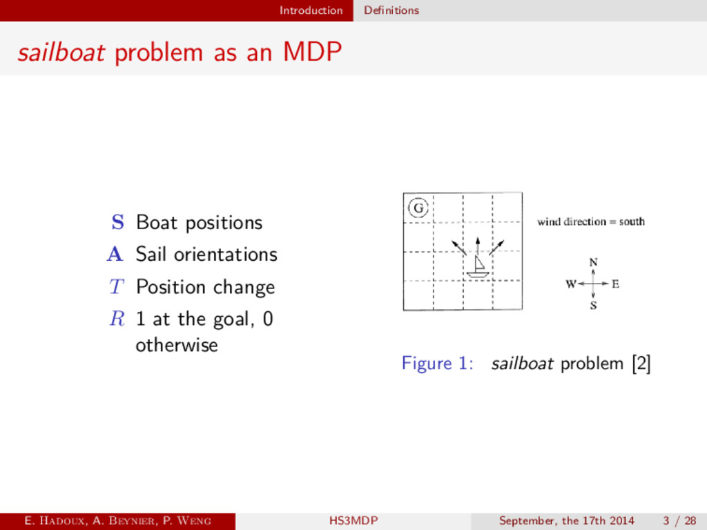
3. Introduction Definitions sailboat problem as an MDP S Boat positions A Sail orientations T Position change R 1 at the goal, 0 otherwise Figure 1: sailboat problem [2] E. Hadoux, A. Beynier, P. Weng HS3MDP September, the 17th 2014 3 / 28
4. Introduction Algorithms on MDPs Algorithms on MDPs T and/or R unknown: Value or Policy iteration unusable Reinforcement learning ⇒ No convergence guarantee with non-stationarity E. Hadoux, A. Beynier, P. Weng HS3MDP September, the 17th 2014 4 / 28
5. Existing models and algorithms 1 Introduction 2 Existing models and algorithms 3 HM-MDPs extension 4 Experimentations 5 Conclusion and perspectives E. Hadoux, A. Beynier, P. Weng HS3MDP September, the 17th 2014 5 / 28
6. Existing models and algorithms HM-MDP Hidden-Mode MDP (HM-MDP) [2] Key idea Non-stationary env. can be seen as a composition of stationary env. HM-MDP Stat. MDPs, linked by a transition function ⇒ M, C , ∀Mi ∈ M, Mi is an MDP S, A, Ti, Ri . M Set of modes C Transition function over modes (C : M → Pr(M)) The new mode is drawn after each decision. Figure 2: 3 modes, 4 states, 1 action HM-MDP [2]. E. Hadoux, A. Beynier, P. Weng HS3MDP September, the 17th 2014 6 / 28
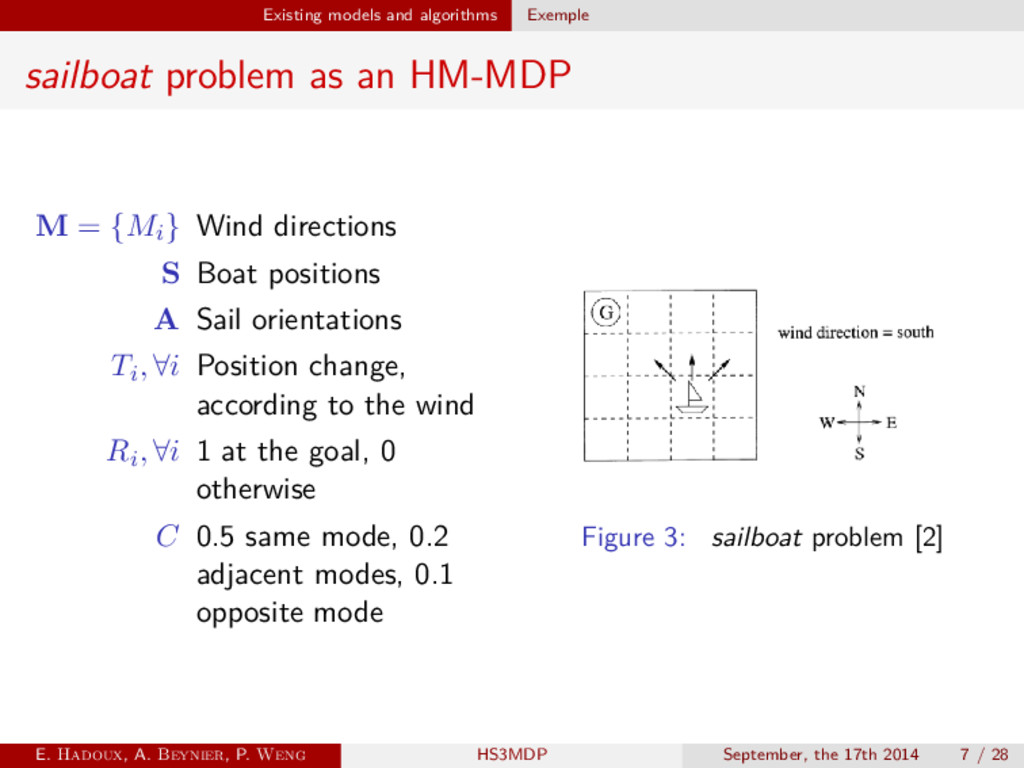
7. Existing models and algorithms Exemple sailboat problem as an HM-MDP M = {Mi} Wind directions S Boat positions A Sail orientations Ti, ∀i Position change, according to the wind Ri, ∀i 1 at the goal, 0 otherwise C 0.5 same mode, 0.2 adjacent modes, 0.1 opposite mode Figure 3: sailboat problem [2] E. Hadoux, A. Beynier, P. Weng HS3MDP September, the 17th 2014 7 / 28
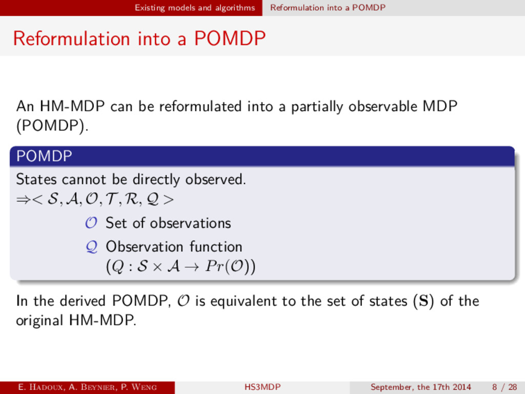
8. Existing models and algorithms Reformulation into a POMDP Reformulation into a POMDP An HM-MDP can be reformulated into a partially observable MDP (POMDP). POMDP States cannot be directly observed. ⇒< S, A, O, T , R, Q > O Set of observations Q Observation function (Q : S × A → Pr(O)) In the derived POMDP, O is equivalent to the set of states (S) of the original HM-MDP. E. Hadoux, A. Beynier, P. Weng HS3MDP September, the 17th 2014 8 / 28
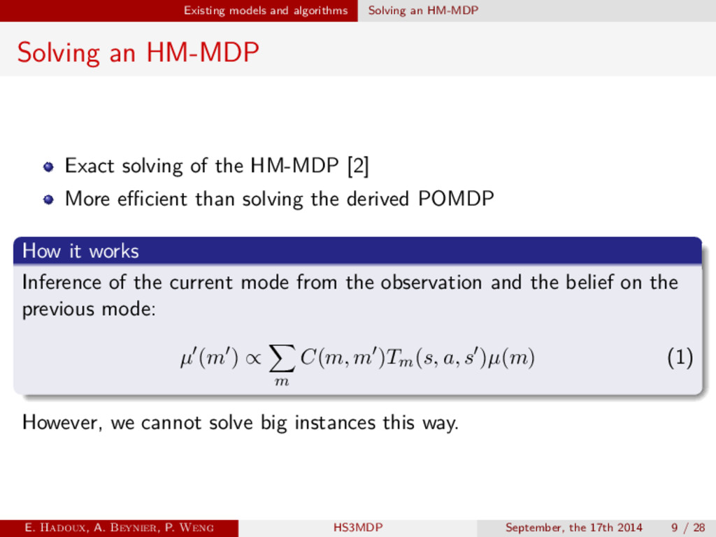
9. Existing models and algorithms Solving an HM-MDP Solving an HM-MDP Exact solving of the HM-MDP [2] More efficient than solving the derived POMDP How it works Inference of the current mode from the observation and the belief on the previous mode: µ (m ) ∝ m C(m, m )Tm(s, a, s )µ(m) (1) However, we cannot solve big instances this way. E. Hadoux, A. Beynier, P. Weng HS3MDP September, the 17th 2014 9 / 28
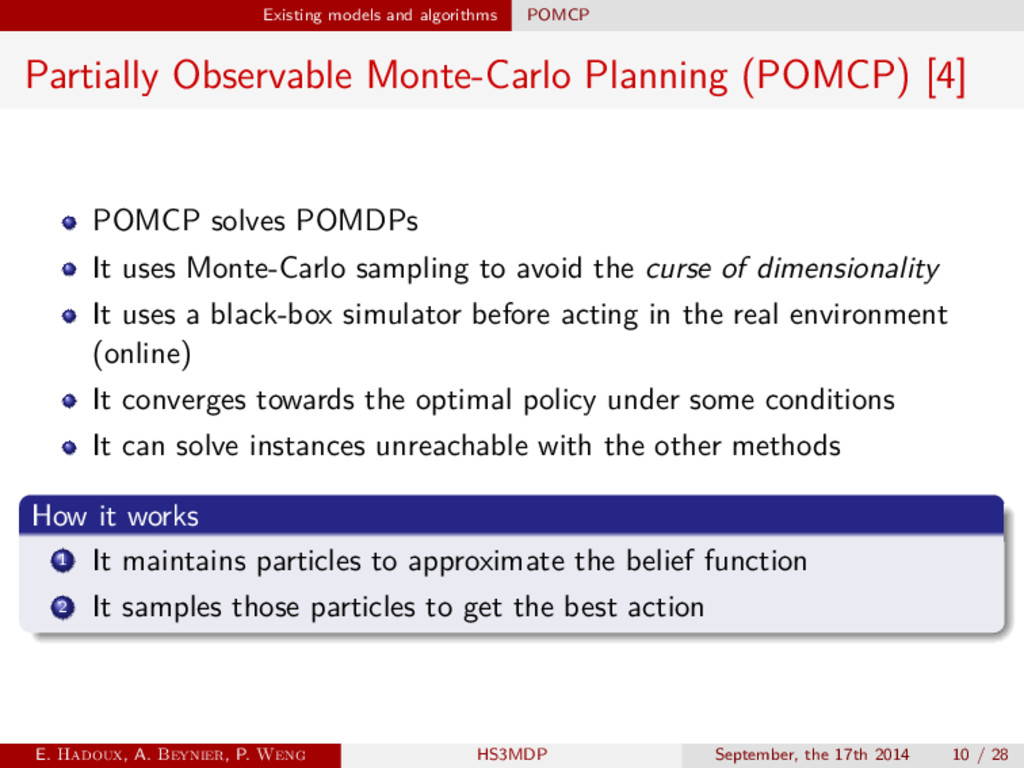
10. Existing models and algorithms POMCP Partially Observable Monte-Carlo Planning (POMCP) [4] POMCP solves POMDPs It uses Monte-Carlo sampling to avoid the curse of dimensionality It uses a black-box simulator before acting in the real environment (online) It converges towards the optimal policy under some conditions It can solve instances unreachable with the other methods E. Hadoux, A. Beynier, P. Weng HS3MDP September, the 17th 2014 10 / 28
11. Existing models and algorithms POMCP Partially Observable Monte-Carlo Planning (POMCP) [4] POMCP solves POMDPs It uses Monte-Carlo sampling to avoid the curse of dimensionality It uses a black-box simulator before acting in the real environment (online) It converges towards the optimal policy under some conditions It can solve instances unreachable with the other methods How it works 1 It maintains particles to approximate the belief function 2 It samples those particles to get the best action E. Hadoux, A. Beynier, P. Weng HS3MDP September, the 17th 2014 10 / 28
12. HM-MDPs extension 1 Introduction 2 Existing models and algorithms 3 HM-MDPs extension 4 Experimentations 5 Conclusion and perspectives E. Hadoux, A. Beynier, P. Weng HS3MDP September, the 17th 2014 11 / 28
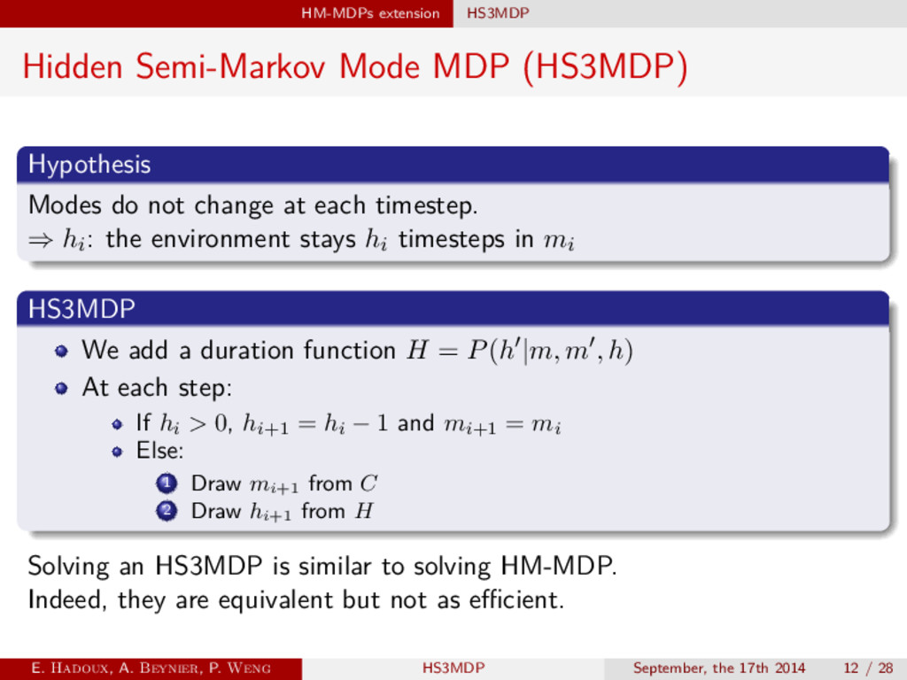
13. HM-MDPs extension HS3MDP Hidden Semi-Markov Mode MDP (HS3MDP) Hypothesis Modes do not change at each timestep. ⇒ hi: the environment stays hi timesteps in mi HS3MDP We add a duration function H = P(h |m, m , h) At each step: If hi > 0, hi+1 = hi − 1 and mi+1 = mi Else: 1 Draw mi+1 from C 2 Draw hi+1 from H Solving an HS3MDP is similar to solving HM-MDP. Indeed, they are equivalent but not as efficient. E. Hadoux, A. Beynier, P. Weng HS3MDP September, the 17th 2014 12 / 28
14. HM-MDPs extension Solving an HS3MDP with POMCP Solving an HS3MDP with POMCP Original method: Lack of particles with big states space E. Hadoux, A. Beynier, P. Weng HS3MDP September, the 17th 2014 13 / 28
15. HM-MDPs extension Solving an HS3MDP with POMCP Solving an HS3MDP with POMCP Original method: Lack of particles with big states space Adding more particles implies doing more simulations E. Hadoux, A. Beynier, P. Weng HS3MDP September, the 17th 2014 13 / 28
16. HM-MDPs extension Solving an HS3MDP with POMCP Solving an HS3MDP with POMCP Original method: Lack of particles with big states space Adding more particles implies doing more simulations Our solution: Replace particles drawing by drawing a belief state from µ(m, h) E. Hadoux, A. Beynier, P. Weng HS3MDP September, the 17th 2014 13 / 28
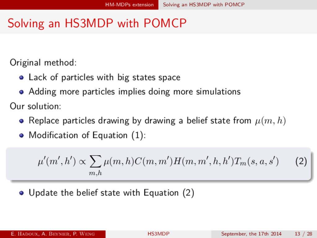
17. HM-MDPs extension Solving an HS3MDP with POMCP Solving an HS3MDP with POMCP Original method: Lack of particles with big states space Adding more particles implies doing more simulations Our solution: Replace particles drawing by drawing a belief state from µ(m, h) Modification of Equation (1): µ (m , h ) ∝ m,h µ(m, h)C(m, m )H(m, m , h, h )Tm(s, a, s ) (2) E. Hadoux, A. Beynier, P. Weng HS3MDP September, the 17th 2014 13 / 28
18. HM-MDPs extension Solving an HS3MDP with POMCP Solving an HS3MDP with POMCP Original method: Lack of particles with big states space Adding more particles implies doing more simulations Our solution: Replace particles drawing by drawing a belief state from µ(m, h) Modification of Equation (1): µ (m , h ) ∝ m,h µ(m, h)C(m, m )H(m, m , h, h )Tm(s, a, s ) (2) Update the belief state with Equation (2) E. Hadoux, A. Beynier, P. Weng HS3MDP September, the 17th 2014 13 / 28
19. Experimentations 1 Introduction 2 Existing models and algorithms 3 HM-MDPs extension 4 Experimentations 5 Conclusion and perspectives E. Hadoux, A. Beynier, P. Weng HS3MDP September, the 17th 2014 14 / 28
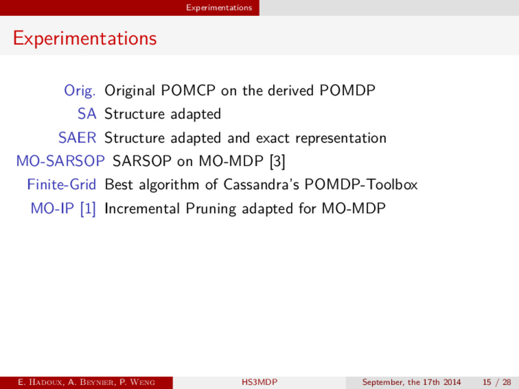
20. Experimentations Experimentations Orig. Original POMCP on the derived POMDP SA Structure adapted SAER Structure adapted and exact representation MO-SARSOP SARSOP on MO-MDP [3] Finite-Grid Best algorithm of Cassandra’s POMDP-Toolbox MO-IP [1] Incremental Pruning adapted for MO-MDP E. Hadoux, A. Beynier, P. Weng HS3MDP September, the 17th 2014 15 / 28
21. Experimentations Sailboat Results for sailboat Sim. Orig. SA SAER MO-SARSOP 1 60 11.7% 6.7% 408.3% 2 63 30.2% 30.2% 384.1% 4 55 38.2% 54.5% 454.5% 8 70 8.6% 27.1% 335.7% 16 59 13.6% 88.1% 416.9% 32 66 28.8% 92.4% 362.1% 64 90 21.1% 45.6% 238.9% 128 94 53.2% 71.3% 224.5% 256 119 48.7% 76.5% 156.3% 512 159 31.4% 27.0% 91.8% 1024 177 20.9% 28.8% 72.3% 2048 206 13.6% 10.2% 48.1% 4096 226 12.4% 16.4% 35.0% 8192 227 20.7% 25.6% 34.4% E. Hadoux, A. Beynier, P. Weng HS3MDP September, the 17th 2014 16 / 28
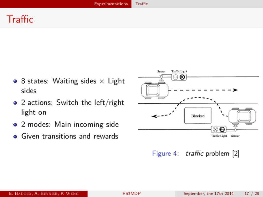
22. Experimentations Traffic Traffic 8 states: Waiting sides × Light sides 2 actions: Switch the left/right light on 2 modes: Main incoming side Given transitions and rewards Figure 4: traffic problem [2] E. Hadoux, A. Beynier, P. Weng HS3MDP September, the 17th 2014 17 / 28
23. Experimentations Traffic Results for traffic Sim. Orig. SA SAER Opt. 1 -3.42 0.0% 0.0% 38.5% 2 -2.86 3.0% 4.0% 26.5% 4 -2.80 8.1% 8.8% 25.0% 8 -2.68 6.0% 9.4% 21.7% 16 -2.60 8.0% 8.0% 19.2% 32 -2.45 5.3% 6.9% 14.3% 64 -2.47 10.0% 9.1% 14.9% 128 -2.34 4.3% 3.4% 10.4% 256 -2.41 8.5% 10.5% 12.7% 512 -2.32 5.6% 4.7% 9.3% 1024 -2.31 5.1% 7.0% 9.3% 2048 -2.38 9.0% 10.5% 11.8% Table 2: Results for traffic, Opt. stands for Finite Grid, MO-IP and MO-SARSOP E. Hadoux, A. Beynier, P. Weng HS3MDP September, the 17th 2014 18 / 28
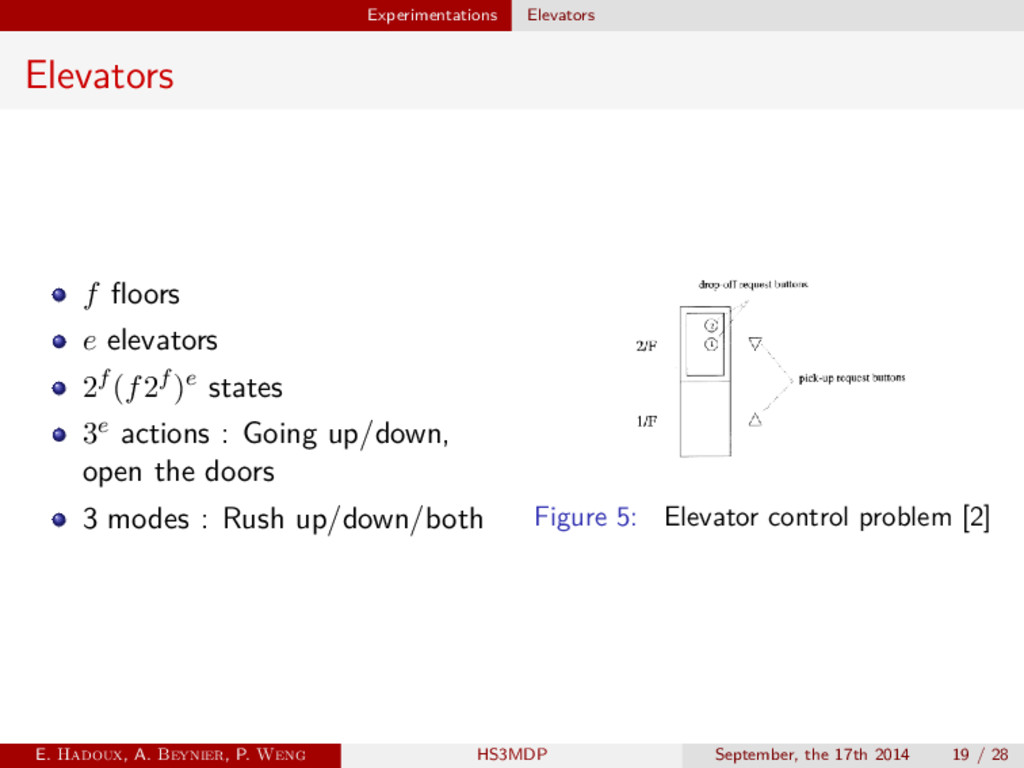
24. Experimentations Elevators Elevators f floors e elevators 2f (f2f )e states 3e actions : Going up/down, open the doors 3 modes : Rush up/down/both Figure 5: Elevator control problem [2] E. Hadoux, A. Beynier, P. Weng HS3MDP September, the 17th 2014 19 / 28
25. Experimentations Elevators Results for elevators Sim. Orig. SA SAER 1 -10.56 0.0% 1.1% 2 -10.60 0.0% 0.0% 4 -10.50 2.2% 3.6% 8 -10.49 4.2% 3.9% 16 -10.44 5.2% 5.0% 32 -10.54 6.2% 6.2% Table 3: Results for f = 7 and e = 1 E. Hadoux, A. Beynier, P. Weng HS3MDP September, the 17th 2014 20 / 28
26. Experimentations Elevators Results for elevators Sim. Orig. SA SAER 1 -7.41 1.0% 0.4% 2 -7.35 0.3% 0.0% 4 -7.44 1.5% 1.3% 8 -7.35 0.4% 0.0% 16 -7.30 19.1% 17.2% 32 -7.25 22.1% 21.6% 64 -7.17 24.3% 24.3% 128 -7.22 27.0% 27.0% Table 4: Results for f = 4 and e = 2 E. Hadoux, A. Beynier, P. Weng HS3MDP September, the 17th 2014 21 / 28
27. Experimentations Random environments Random environments Fixed number of states, modes and actions Random transition and reward functions with conditions E. Hadoux, A. Beynier, P. Weng HS3MDP September, the 17th 2014 22 / 28
28. Experimentations Random environments Results for random environments Sim. Orig. SA SAER 1 0.41 0.0% 5.6% 2 0.41 4.9% 51.4% 4 0.42 11.5% 140.9% 8 0.44 30.9% 209.6% 16 0.48 34.6% 234.7% 32 0.58 46.0% 223.0% 64 0.77 53.1% 187.2% 128 1.08 45.7% 123.4% 256 1.52 33.5% 70.0% 512 1.98 19.6% 34.5% 1024 2.30 12.5% 17.3% Table 5: Results with ns = 50, na = 5 and nm = 5 E. Hadoux, A. Beynier, P. Weng HS3MDP September, the 17th 2014 23 / 28
29. Experimentations Random environments Results for random environments Sim. Orig. SA SAER 1 0.39 0.1% 8.9% 2 0.39 21.0% 57.5% 4 0.40 9.9% 149.0% 8 0.41 24.0% 224.6% 16 0.43 33.0% 261.3% 32 0.48 58.2% 275.8% 64 0.60 76.2% 248.7% 128 0.83 75.4% 184.5% 256 1.16 64.1% 115.9% 512 1.61 41.5% 61.5% 1024 2.05 2.2% 28.8% Table 6: Results with ns = 50, na = 5 and nm = 10 E. Hadoux, A. Beynier, P. Weng HS3MDP September, the 17th 2014 24 / 28
30. Experimentations Random environments Results for random environments Sim. Orig. SA SAER 1 0.39 0.8% 11.9% 2 0.40 2.6% 51.1% 4 0.40 2.7% 138.9% 8 0.41 11.8% 225.2% 16 0.41 22.3% 270.8% 32 0.45 42.9% 290.3% 64 0.51 77.5% 305.5% 128 0.63 102.2% 261.1% 256 0.85 102.7% 186.8% 512 1.23 73.3% 107.7% 1024 1.66 43.6% 55.3% Table 7: Results with ns = 50, na = 5 and nm = 20 E. Hadoux, A. Beynier, P. Weng HS3MDP September, the 17th 2014 25 / 28
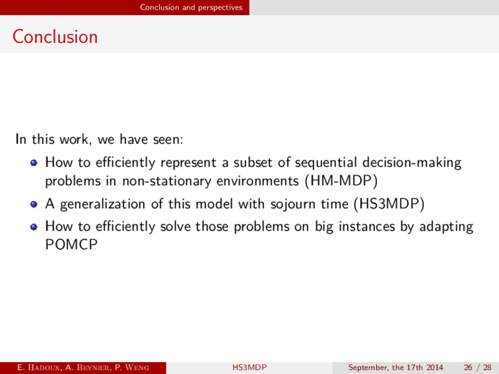
31. Conclusion and perspectives Conclusion In this work, we have seen: How to efficiently represent a subset of sequential decision-making problems in non-stationary environments (HM-MDP) A generalization of this model with sojourn time (HS3MDP) How to efficiently solve those problems on big instances by adapting POMCP E. Hadoux, A. Beynier, P. Weng HS3MDP September, the 17th 2014 26 / 28
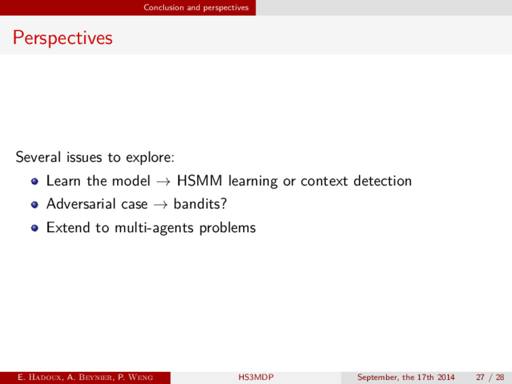
32. Conclusion and perspectives Perspectives Several issues to explore: Learn the model → HSMM learning or context detection Adversarial case → bandits? Extend to multi-agents problems E. Hadoux, A. Beynier, P. Weng HS3MDP September, the 17th 2014 27 / 28
33. Conclusion and perspectives References Mauricio Araya-López, Vincent Thomas, Olivier Buffet, and François Charpillet. A closer look at MOMDPs. In International Conference on Tools with Artificial Intelligence (ICTAI), 2010. Samuel Ping-Man Choi. Reinforcement learning in nonstationary environments. PhD thesis, Hong Kong University of Science and Technology, 2000. Sylvie C.W. Ong, Shao Wei Png, David Hsu, and Wee Sun Lee. POMDPs for robotic tasks with mixed observability. In Robotics: Science & Systems, 2009. David Silver and Joel Veness. Monte-Carlo planning in large POMDPs. In NIPS, pages 2164–2172, 2010. E. Hadoux, A. Beynier, P. Weng HS3MDP September, the 17th 2014 28 / 28