Upgrade to Pro — share decks privately, control downloads, hide ads and more …

ESRF tutorial: 3-D image processing with scikit-image

ESRF tutorial: 3-D image processing with scikit-image

A presentation of the scikit-image library and how to use it to process 3-D data

Emmanuelle Gouillart

February 08, 2016
Tweet

More Decks by Emmanuelle Gouillart

Other Decks in Science

Transcript

  1. 3-D image processing with scikit-image and the scientic Python ecosystem

    Emmanuelle Gouillart joint Unit CNRS/Saint-Gobain SVI @EGouillart scikit-image team
  2. What is scikit-image? An open-source (BSD) generic image processing library

    for the Python language (and NumPy data arrays)
  3. What is scikit-image? An open-source (BSD) generic image processing library

    for the Python language (and NumPy data arrays) for 2D & 3D images simple API & gentle learning curve
  4. Python: a versatile & modern language A modern language (1989)

    concise interpreted >>> f o r i in range (3): ... p r i n t ( i **2) ... 0 1 4 x xkcd.com
  5. Python: a versatile & modern language A modern language (1989)

    concise interpreted >>> f o r i in range (3): ... p r i n t ( i **2) ... 0 1 4 x used by various actors web dev scripting scientific computing synchrotrons education... xkcd.com
  6. NumpPy: Python objects for numerical arrays Multi-dimensional numerical data container

    (based on compiled code) + utility functions to create/manipulate them >>> a = np.random. r a n d o m i n t e g e r s (0, 1, (2, 2, 2)) >>> a a r r a y ([[[0 , 1], [1, 0]], [[0, 0], [0, 1]]]) >>> a. shape , a. dtype ((2, 2, 2), dtype ( ’ int64 ’ )) x
  7. NumpPy: Python objects for numerical arrays Multi-dimensional numerical data container

    (based on compiled code) + utility functions to create/manipulate them >>> a = np.random. r a n d o m i n t e g e r s (0, 1, (2, 2, 2)) >>> a a r r a y ([[[0 , 1], [1, 0]], [[0, 0], [0, 1]]]) >>> a. shape , a. dtype ((2, 2, 2), dtype ( ’ int64 ’ )) x Efficient and versatile data access indexing and slicing fancy indexing
  8. First steps with scikit-image >>> from skimage import data ,

    measure >>> im = data . b i n a r y b l o b s (128 , n dim =3, v o l u m e f r a c t i o n =0.2) >>> im. shape # 3-D array (128 , 128, 128) >>> l a b e l s = measure . l a b e l (im) >>> type(im), type( l a b e l s ) # images are numpy arrays (<type ’numpy . ndarray ’ >, <type ’numpy . ndarray ’ >) >>> l a b e l s [0, 0, 0] # pixels are array elements 0 x Visualization with Mayavi [Ramachandran and Varoquaux, 2011] Images are NumPy arrays Pixels are array elements Simple API relying on functions new = function(image) Most functions work for 2D & 3D Optional parameters: keyword arguments
  9. Datasheet Package statistics http://scikit-image.org/ Release 0.11 (1 - 2 release

    per year) 0.12 coming this month! (02/16) Among 1000 best packages on PyPi Development model Mature algorithms Only Python + Cython code for easier maintainability Focus on good practices: testing, documentation, version control Hosted on GitHub: thorough code reivew + continuous integration Core team of 5 − 10 persons ∼ 50 contributors / release
  10. API of scikit-image skimage filters restoration segmentation ... denoise_bilateral input

    array + optional parameters output (array) submodule module function variables
  11. Denoising tomography images Data from ESRF, ID19 In-situ imaging of

    phase separation in silicate melts [Bouttes et al., 2014, Bouttes et al., 2015] From basic (generic) to advanced (specific) filters
  12. Denoising tomography images Histogram of pixel values From basic (generic)

    to advanced (specific) filters bilateral = restoration . denoise bilateral (dat) bilateral = restoration . denoise bilateral (dat, sigma range=2.5, sigma spatial=2) tv = restoration . denoise tv chambolle (dat, weight=0.5)
  13. Example: segmentation of low-constrast regions In-situ imaging of glass batch

    reactive melting [Gouillart et al., 2012] Non-local means denoising to preserve texture Histogram-based markers extraction Random walker segmentation Non-local means: average similar patches [Buades et al., 2005] Random walker:anisotropic diffusion from markers [Grady, 2006] Random walker less sensitive to noise than watershed, but slower
  14. Mathematical morphology skimage.morphology: binary + grayscale morphology dilation, erosion, closing,

    opening several structural elements remove small objects watershed
  15. Feature extraction followed by classification Combining scikit-image and scikit-learn Extract

    features (skimage.feature) Pixels intensity values (R, G, B) Local gradients More advanced descriptors: HOGs, Gabor, ... Train classifier with known regions here, random forest classifier Classify pixels
  16. Other modules skimage.transform: geometrical transformations scale, zoom, rotate, swirl, warp,

    ... skimage.exposure: manipulate range of color/grayscales . . .
  17. Goodies from the ecosystem IPython notebook: code, text, interactive widgets...

    http://tonysyu.github.io/ ipython-jupyter-widgets-an-image-convolution-demo.html
  18. Goodies from the ecosystem joblib: easy simple parallel computing +

    lazy re-evaluation >>> from j o b l i b import P a r a l l e l , d e l a y e d >>> from math import s q r t >>> P a r a l l e l ( n j o b s =1)( d e l a y e d ( s q r t )( i **2) f o r i in range (10)) [0.0 , 1.0, 2.0, 3.0, 4.0, 5.0, 6.0, 7.0, 8.0, 9.0] x Familiar with this mess? from skimage import f i l t e r s # Comment to save some time # filter_im = filters.median(im) # binary_im = filters. threshold_otsu (filter_im) v a l u e s = np. unique (im) x
  19. Goodies from the ecosystem joblib: easy simple parallel computing +

    lazy re-evaluation Familiar with this mess? from skimage import f i l t e r s # Comment to save some time # filter_im = filters.median(im) # binary_im = filters. threshold_otsu (filter_im) v a l u e s = np. unique (im) x >>> from j o b l i b import Memory >>> mem = Memory( c a c h e d i r = ’ /tmp/ j o b l i b ’ ) >>> square = mem. cache (np. square ) >>> b = square (a) [Memory] C a l l i n g square ... square ( a r r a y ([[ 0., 0., 1.], [ 1., 1., 1.], [ 4., 2., 1.]])) s q u a r e - 0... s , 0.0 min >>> c = square (a) >>> # The above call did not trigger an evaluation x
  20. A few tricks for large images I/O: tomography images might

    not fit into memory use memory mapping of different file formats (raw binary with NumPy, hdf5 with pytables) for input data, and intermediate results Divide into blocks: use util.view as blocks to iterate conveniently over blocks Use NumPy wisely: slicing over an array makes no copy
  21. Wish list and work in progress Port to 3-D a

    few only 2-D functions: region properties, clear border in 0.12 skeletonization in 0.13dev Option for embarassingly-parallel processing of image blocks Experimental feature in 0.12 graph cut segmentation ... your suggestions?
  22. Bibliography I Bouttes, D., Gouillart, E., Boller, E., Dalmas, D.,

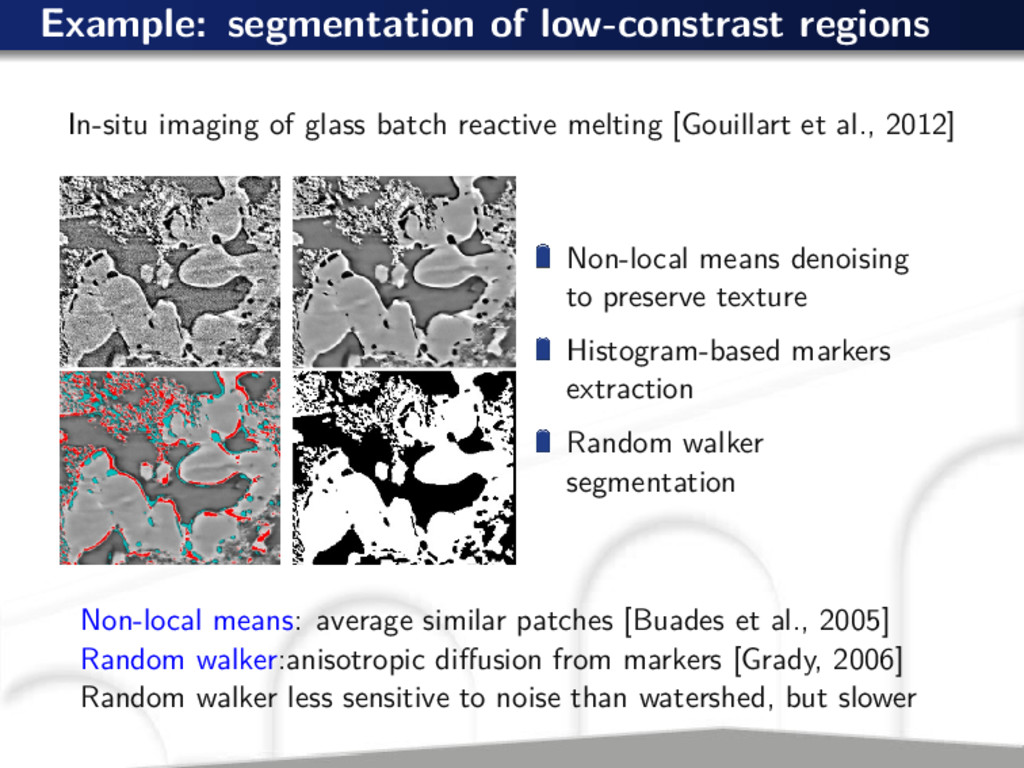
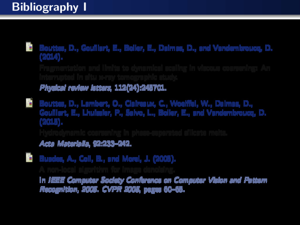
    and Vandembroucq, D. (2014). Fragmentation and limits to dynamical scaling in viscous coarsening: An interrupted in situ x-ray tomographic study. Physical review letters, 112(24):245701. Bouttes, D., Lambert, O., Claireaux, C., Woelffel, W., Dalmas, D., Gouillart, E., Lhuissier, P., Salvo, L., Boller, E., and Vandembroucq, D. (2015). Hydrodynamic coarsening in phase-separated silicate melts. Acta Materialia, 92:233–242. Buades, A., Coll, B., and Morel, J. (2005). A non-local algorithm for image denoising. In IEEE Computer Society Conference on Computer Vision and Pattern Recognition, 2005. CVPR 2005, pages 60–65.
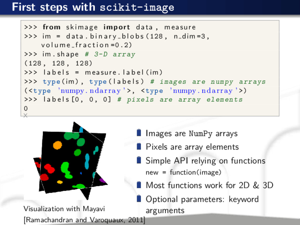
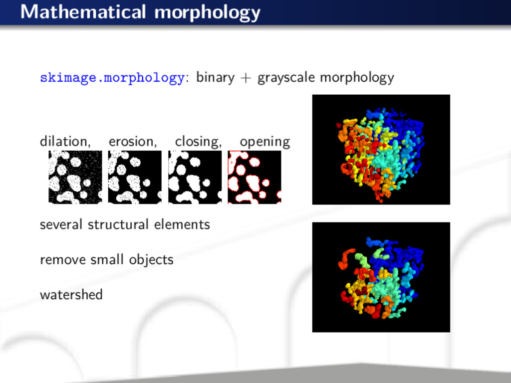
  23. Bibliography II Gouillart, E., Toplis, M. J., Grynberg, J., Chopinet,

    M.-H., Sondergard, E., Salvo, L., Su´ ery, M., Di Michiel, M., and Varoquaux, G. (2012). In situ synchrotron microtomography reveals multiple reaction pathways during soda-lime glass synthesis. Journal of the American Ceramic Society, 95(5):1504–1507. Grady, L. (2006). Random walks for image segmentation. IEEE Transactions on Pattern Analysis and Machine Intelligence, pages 1768–1783. Ramachandran, P. and Varoquaux, G. (2011). Mayavi: 3d visualization of scientific data. Computing in Science & Engineering, 13(2):40–51.