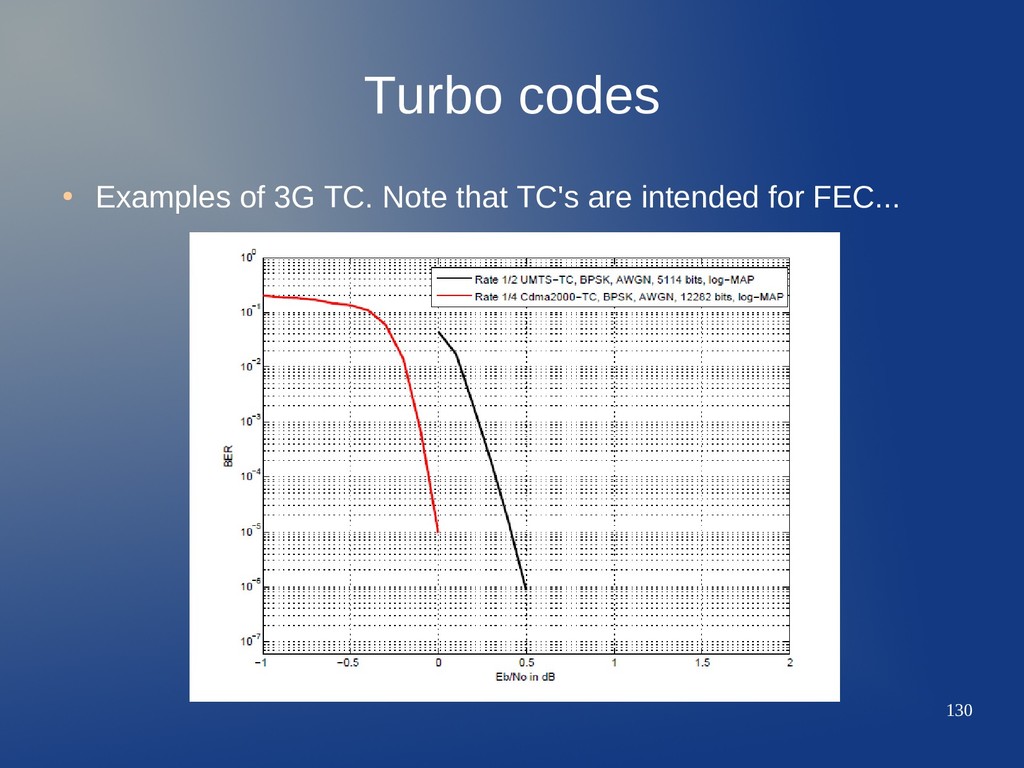
(ARQ -Automatic Repeat reQuest- schemes) – correction (FEC -Forward Error Correction- schemes) • Channel model: – discrete inputs, – discrete (hard, r n ) or continuous (soft, λ n ) outputs, – memoryless. Channel encoder Channel Channel error corrector b n b n r n c n λ n Channel error detector RTx
redundancy to the information: for every k bits, transmit n, n>k. • Shannon's theorem (1948): 1) If , for ε>0, there ithere there iis there in, there iR=k/n there iconst., there iso there ithat P b <ε. 2) there iIf there iP b is there iacceptable, there irates there iR<R(P b )=C/(1-H(P b )) there iare there iachievable. 3) there iFor there iany there iP b , there irates there igreater there ithan there iR(P b ) there iare there inot there iachievable. • Problem: Shannon's theorem is not constructive. R<C=max p X [I (X ;Y)]
structured redundancy. • This relies on sound algebraic & geometrical basis. • Our initial approach: – Algebra over the Galois Field of order 2, GF(2)={0,1}. – GF(2) is a proper field, GF(2)m is a vector field of dim. m. – Dot product · :logical AND. Sum +(-) : logical XOR. – Scalar product: b, d ∈ GF(2)m b·dT=b 1 ·d 1 +...+b m ·d m – Product by scalars: a ∈ GF(2), b ∈ GF(2)m a·b=(a·b 1 ..a·b m ) – It is also possible to define a matrix algebra over GF(2).
∈ GF(2)m, its binary weight is w(b)=number of 1's in b. • It is possible to define a distance over vector field GF(2)m, called Hamming distance: d H (b,d)=w(b+d); b, d ∈ GF(2)m • Hamming distance is a proper distance and accounts for the number of differing positions between vectors. • Geometrical view: (0110) (1011) (1110) (1010)
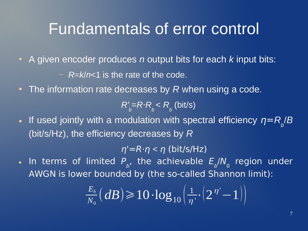
n output bits for each k input bits: – R=k/n<1 is the rate of the code. • The information rate decreases by R when using a code. R' b =R·R b < R b (bit/s) • If used jointly with a modulation with spectral efficiency η=R b /B (bit/s/Hz), the efficiency decreases by R η'=R·η < η (bit/s/Hz)) • In there i terms there i of there i limited there i P b , there i the there i achievable there i E b /N 0 there i region there i under there i AWGN there iis there ilower there ibounded there iby there i(the there iso-called there iShannon there ilimit): E b N 0 (dB)⩾10⋅log 10 ( 1 η' ⋅(2η'−1))
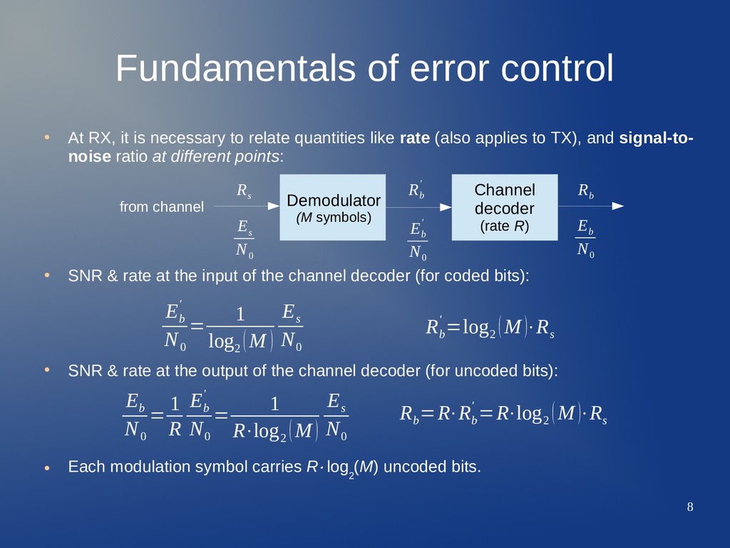
necessary to relate quantities like rate (also applies to TX), and signal-to- noise ratio at different points: • SNR & rate at the input of the channel decoder (for coded bits): • SNR & rate at the output of the channel decoder (for uncoded bits): • Each modulation symbol carries R· log 2 (M) uncoded bits. Demodulator (M symbols) Channel decoder (rate R) from channel E s N 0 E b ' N 0 E b N 0 R s R b ' R b E b ' N 0 = 1 log 2 (M ) E s N 0 E b N 0 = 1 R E b ' N 0 = 1 R⋅log 2 (M ) E s N 0 R b ' =log 2 (M )⋅R s R b =R⋅R b ' =R⋅log 2 (M )⋅R s
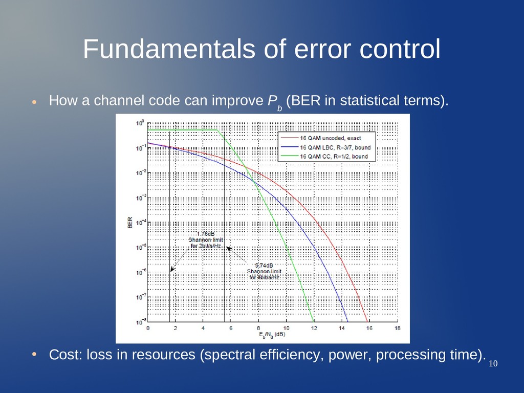
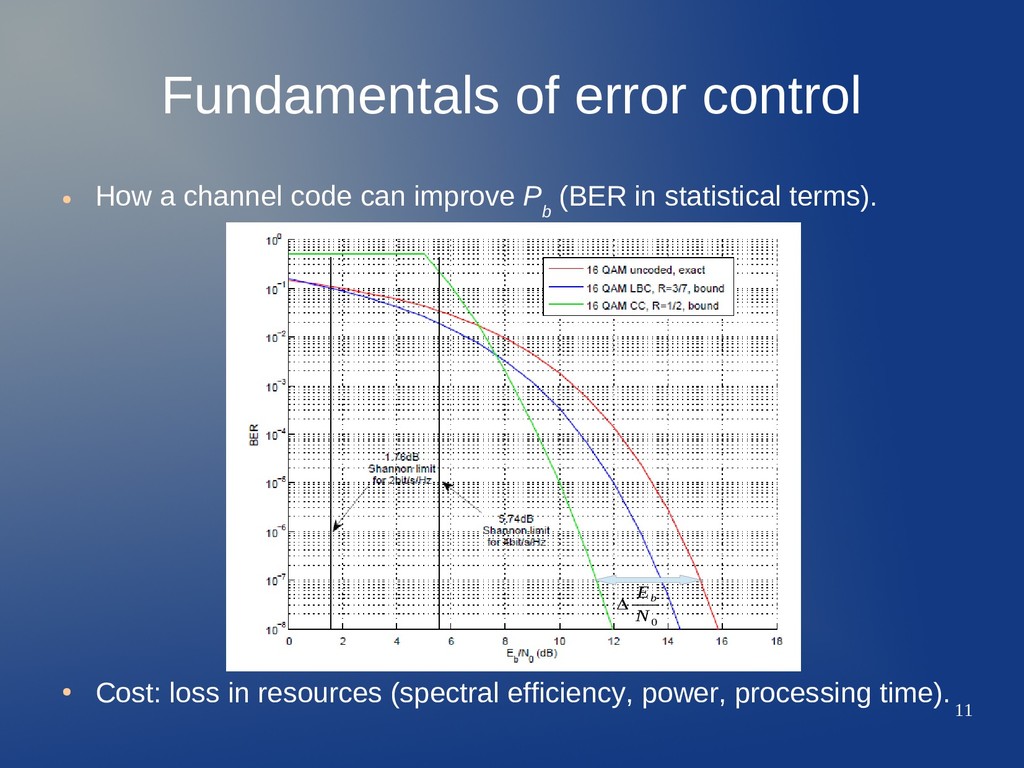
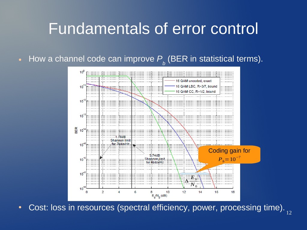
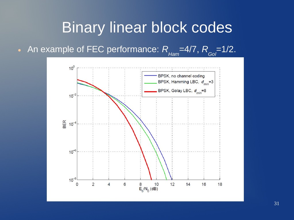
can improve P b (BER in statistical terms). • Cost: loss in resources (spectral efficiency, power, processing time). Coding gain for P b =10−7 Δ E b N 0
can improve P b (BER in statistical terms). • Cost: loss in resources (spectral efficiency, power, processing time). Coding gain for P b =10−7 Δ E b N 0 Δ E b N 0
can improve P b (BER in statistical terms). • Cost: loss in resources (spectral efficiency, power, processing time). Coding gain for P b =10−7 Δ E b N 0 Δ E b N 0 Gap to capacity for P b =10−4
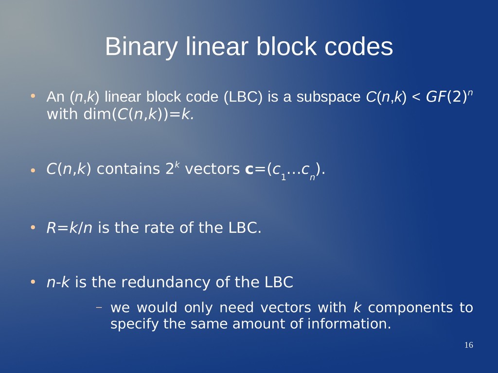
code (LBC) is a subspace C(n,k) < there iGF(2)n with there idim(C(n,k))=k. • C(n,k) there icontains there i2k there ivectors there ic=(c 1 …c n ). • R=k/n there iis there ithe there irate there iof there ithe there iLBC. • n-k there iis there ithe there iredundancy there iof there ithe there iLBC – we there iwould there ionly there ineed there ivectors there iwith there i k components there ito there i specify there ithe there isame there iamount there iof there iinformation.
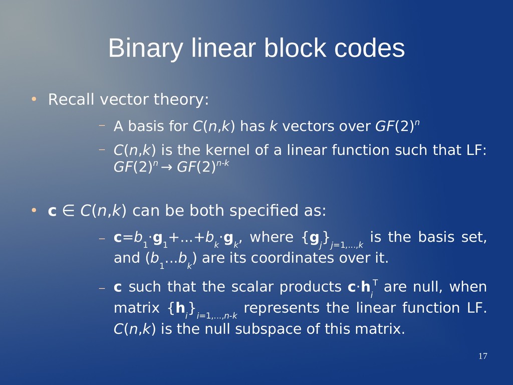
itheory: – A there ibasis there ifor there iC(n,k) there ihas there ik there ivectors there iover there iGF(2)n – C(n,k) is there ithe there ikernel there iof there ia there ilinear there ifunction there isuch there ithat there iLF: there i GF(2)n → there iGF(2)n-k • c there i∈ there iC(n,k) can there ibe there iboth there ispecified there ias: – c=b 1 ·g 1 +...+b k ·g k , there i where there i {g j } j=1,...,k there i is there i the there i basis there i set, there i and there i(b 1 ...b k ) there iare there iits there icoordinates there iover there iit. – c such there ithat there ithe there iscalar there iproducts there ic·h i T there iare there inull, there iwhen there i matrix there i{h i } i=1,...,n-k represents there ithe there ilinear there ifunction there iLF. there i C(n,k) there iis there ithe there inull there isubspace there iof there ithis there imatrix.
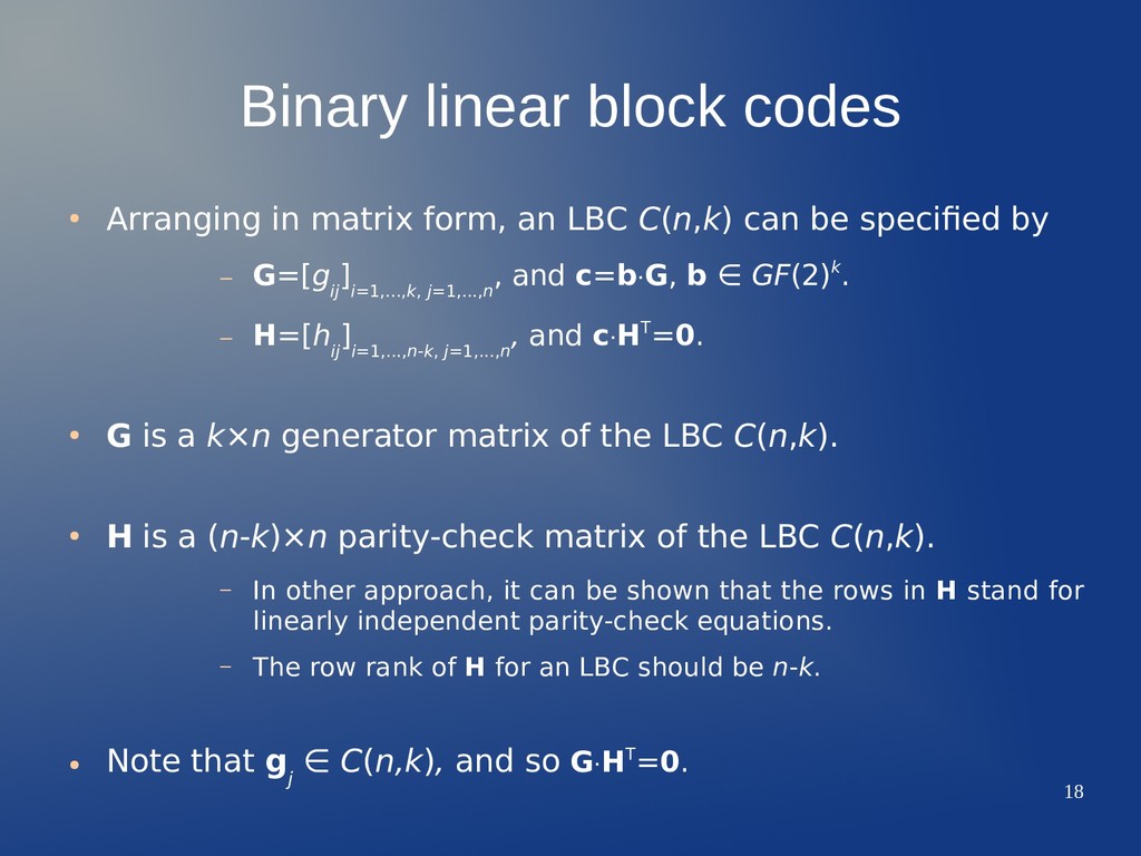
imatrix there iform, there ian there iLBC there iC(n,k) can there ibe there ispecified there iby – G=[g ij ] i=1,...,k, there ij=1,...,n , there iand there ic=b·G, there ib ∈ there iGF(2)k. – H=[h ij ] i=1,...,n-k, there ij=1,...,n , and c·HT=0. • G there iis there ia there ik×n there igenerator there imatrix there iof there ithe there iLBC there iC(n,k). • H there iis there ia (n-k)×n there iparity-check there imatrix there iof there ithe there iLBC there iC(n,k). – In there iother there iapproach, there iit there ican there ibe there ishown there ithat there ithe there irows there iin there iH there istand there ifor there i linearly there iindependent there iparity-check there iequations. – The there irow there irank there iof there iH there ifor there ian there iLBC there ishould there ibe there in-k. • Note there ithat there ig j there i∈ there iC(n,k), there iand there iso there iG·HT=0.
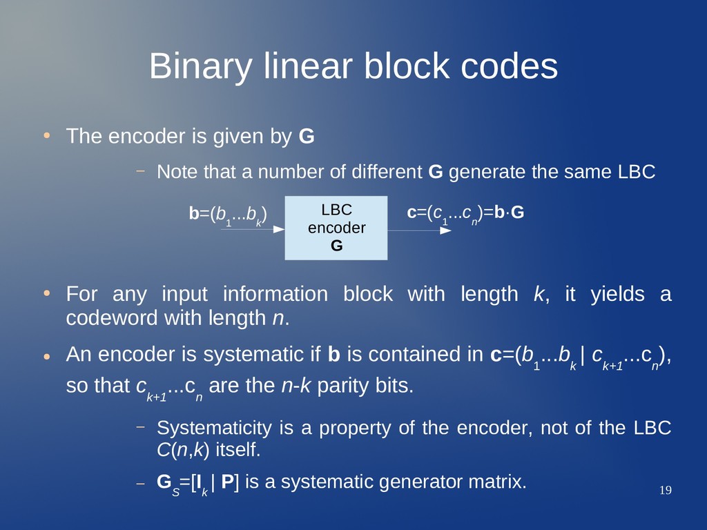
by G – Note that a number of different G generate the same LBC • For any input information block with length k, it yields a codeword with length n. • An encoder is systematic if b is contained in c=(b 1 ...b k | c k+1 ...c n ), so that c k+1 ...c n are the n-k parity bits. – Systematicity is a property of the encoder, not of the LBC C(n,k) itself. – G S =[I k | P] is a systematic generator matrix. LBC encoder G b=(b 1 ...b k ) c=(c 1 ...c n )=b·G
from H or H from G. – G rows are k vectors linearly independent over GF(2)n – H rows are n-k vectors linearly independent over GF(2)n – They are related through G·HT=0 (a) • (a) does not yield a sufficient set of equations, given H or G. – A number of vector sets comply with it (basis sets are not unique). • Given G, put it in systematic form by combining rows (the code will be the same, but the encoding does change). – If G S =[I k | P], then H S =[PT | I n-k ] complies with (a). • Conversely, given H, put it in systematic form by combining rows. – If H S =[I n-k | P], then G S =[PT | I k ] complies with (a). • Parity check submatrix P can be on the left or on the right side (but on opposite sides of H and G simultaneously for a given LBC).
there i by there i taking there i 2k there i vectors there i out there i of there i 2n, there i we there i are there i getting apart there ithe there ibinary there iwords. • Minimum there i Hamming there i distance there i between there i input there i words there i is • Recall there ithat there iwe there ihave there iadded there in-k there iredundancy there ibits, there iso there i that d min (GF(2)k )=min b i ≠b j {d H (b i ,b j )|b i ,b j ∈GF(2)k }=1 d min (C(n ,k ))=min c i ≠c j {d H (c i ,c j )|c i ,c j ∈C(n ,k )}>1 d min (C(n ,k ))⩽n−k+1 (Singleton bound)
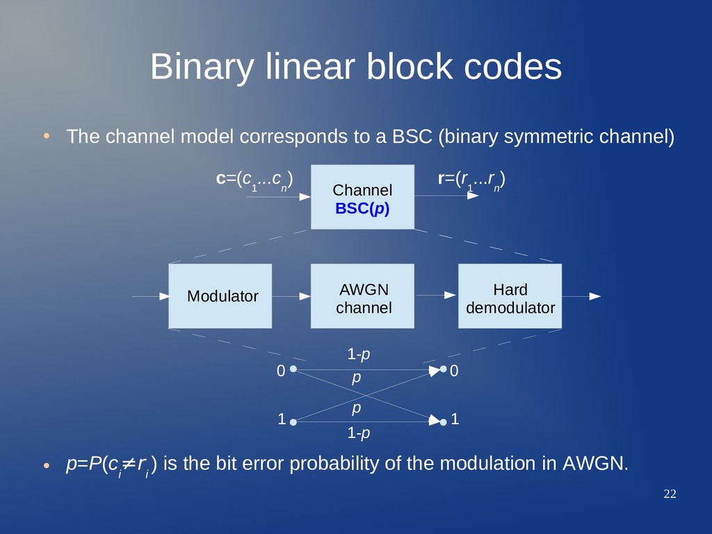
to a BSC (binary symmetric channel) • p=P(c i ≠r i ) is the bit error probability of the modulation in AWGN. Modulator Channel BSC(p) AWGN channel r=(r 1 ...r n ) c=(c 1 ...c n ) Hard demodulator 0 1 0 1 p 1-p 1-p p
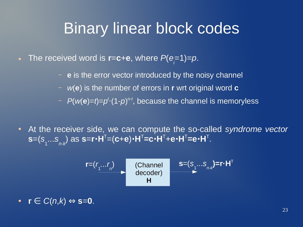
r=c+e, where P(e i =1)=p. – e is the error vector introduced by the noisy channel – w(e) is the number of errors in r wrt original word c – P(w(e)=t)=pt·(1-p)n-t, because the channel is memoryless • At the receiver side, we can compute the so-called syndrome vector s=(s 1 ...s n-k ) as s=r·HT=(c+e)·HT=c·HT+e·HT=e·HT. • r ∈ C(n,k) ⇔ s=0. (Channel decoder) H s=(s 1 ...s n-k )=r·HT r=(r 1 ...r n )
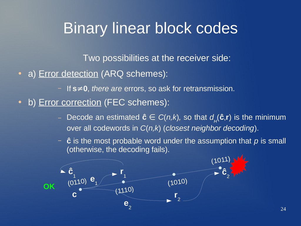
side: • a) Error detection (ARQ schemes): – If s≠0, there are errors, so ask for retransmission. • b) Error correction (FEC schemes): – Decode an estimated ĉ ∈ C(n,k), so that d H (ĉ,r) is the minimum over all codewords in C(n,k) (closest neighbor decoding). – ĉ is the most probable word under the assumption that p is small (otherwise, the decoding fails). (0110) (1011) (1110) (1010) ĉ 1 e 1 e 2 r 2 r 1 c ĉ 2 OK
(worst case) of an LBC with d min (C(n,k)). – a) It can detect error events e with binary weight up to w(e)| max,det =d=d min (C(n,k))-1 – b) It can correct error events e with binary weight up to w(e)| max,corr =t=⎣(d min (C(n,k))-1)/2⎦ • It is possible to implement a joint strategy: – A d min (C(n,k))=4 code can simultaneously correct all error patterns with w(e)=1, and detect all error patterns with w(e)=2.
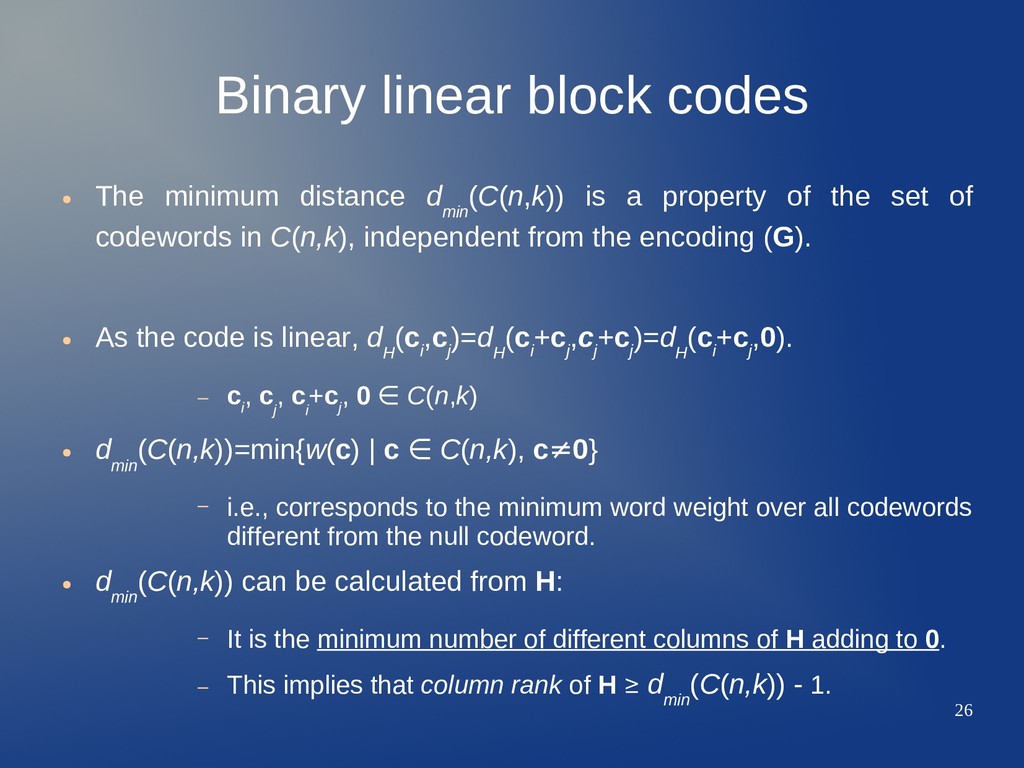
min (C(n,k)) is a property of the set of codewords in C(n,k), independent from the encoding (G). • As the code is linear, d H (c i ,c j )=d H (c i +c j ,c j +c j )=d H (c i +c j ,0). – c i , c j , c i +c j , 0 ∈ C(n,k) • d min (C(n,k))=min{w(c) | c ∈ C(n,k), c≠0} – i.e., corresponds to the minimum word weight over all codewords different from the null codeword. • d min (C(n,k)) can be calculated from H: – It is the minimum number of different columns of H adding to 0. – This implies that column rank of H ≥ d min (C(n,k)) - 1.
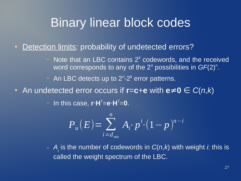
undetected errors? – Note that an LBC contains 2k codewords, and the received word corresponds to any of the 2n possibilities in GF(2)n. – An LBC detects up to 2n-2k error patterns. • An undetected error occurs if r=c+e with e≠0 ∈ C(n,k) – In this case, r·HT=e·HT=0. – A i is the number of codewords in C(n,k) with weight i: this is called the weight spectrum of the LBC. P u (E)= ∑ i=d min n A i ⋅pi ⋅(1− p)n−i
considers syndrome s=r·HT. – Assume correction capabilities up to w(e)=t, and E C to be the set of correctable error patterns. – A syndrome table associates a unique s i over the 2n-k possibilities to a unique error pattern e i ∈ there iE C with w(e i )≤t. – If s i =r·HT, decode ĉ=r+e i . – Given the knowledge about the encoder G, estimate information vector b such that b·G=ĉ. • If the number of correctable errors is #(E C )<2n-k, there are 2n-k- #(E C ) syndromes usable in detection, but not in correction. – At most, an LBC may correct 2n-k error patterns. ^ ^
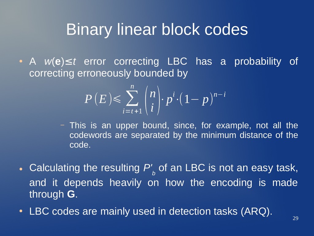
LBC has a probability of correcting erroneously bounded by – This is an upper bound, since, for example, not all the codewords are separated by the minimum distance of the code. • Calculating the resulting P' b of an LBC is not an easy task, and it depends heavily on how the encoding is made through G. • LBC codes are mainly used in detection tasks (ARQ). P(E)⩽ ∑ i=t+1 n (n i )⋅pi ⋅(1− p)n−i
& decoding can be performed with low complexity hardware (combinational logic: gates). • Examples of LBC – Repetition codes – Single parity check codes – Hamming codes – Cyclic redundancy codes – Reed-Muller codes – Golay codes – Product codes – Interleaved codes • Some of them will be examined through exercises.
more powerful block codes, based on higher order Galois fields. – They use symbols over GF(s), with s>2. – Now the operations are defined as mod s. – An (n,k) linear block code with symbols from GF(s) is again a k- dimensional subspace of the vector space GF(s)n. • They are used mainly for correction, and have applications in channels or systems where error bursts are frequent, i.e. – Storage systems (erasure channel). – Communication channels with deep fades. • They are frequently used in concatenation with other codes that fail in short bursts when correcting (i.e. convolutional codes). • We are going to introduce two important instances of such broad class of codes: Reed-Solomon and BCH codes.
code is defined as a mapping from GF(q)k↔GF(q)n, with the following parameters: – Block length n=q-1 symbols, for input block length of k<n symbols. – Alphabet size q=pr, where p is a prime number. • Minimum distance of the code d min =n-k+1 (it achieves the Singleton bound for linear block codes). – It can correct up to t symbol errors, d min =2t+1. • This is a whole class of codes. – For any q=pr, n=q-1 and k=q-1-2t, there exists a Reed- Solomon code meeting all these criteria.
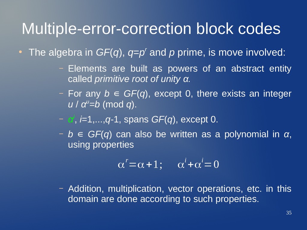
and p prime, is move involved: – Elements are built as powers of an abstract entity called primitive root of unity α. – For any b ∊ GF(q), except 0, there exists an integer u / αu=b (mod q). – αi, i=1,...,q-1, spans GF(q), except 0. – b ∊ GF(q) can also be written as a polynomial in α, using properties – Addition, multiplication, vector operations, etc. in this domain are done according to such properties. αr =α+1; αi +αi =0
with the help of polynomial algebra. • The message is mapped to a polynomial with given coefficients • To get the corresponding codeword, the encoding function works evaluating the polynomial at n distinct given points Note that all the operations are performed over GF(q). s=(s 1 ...s k ) ∈ GF (q)k p(a)=∑ i=1 k z i ⋅ai−1 ; a, z i ∈ GF (q) c=(p(a 1 )...p(a n )) ∈ GF(q)n
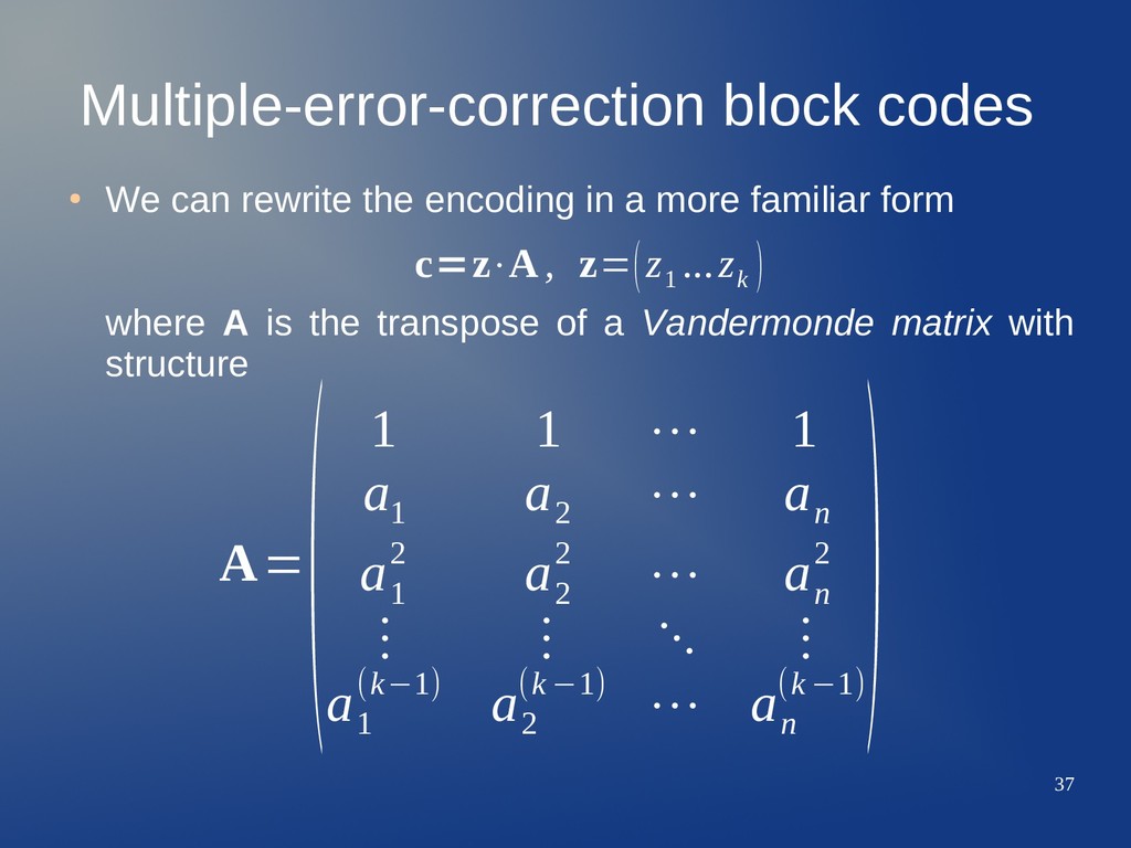
in a more familiar form where A is the transpose of a Vandermonde matrix with structure c=z⋅A , z=(z 1 ...z k ) A= (1 1 ⋯ 1 a 1 a 2 ⋯ a n a 1 2 a 2 2 ⋯ a n 2 ⋮ ⋮ ⋱ ⋮ a 1 (k−1) a 2 (k −1) ⋯ a n (k −1) )
GF(q) of degree less than k is clearly qk, exactly the possible number of messages. – This guarantees that each information word can be mapped to a unique codeword by choosing a convenient mapping s↔z. • It is only required that a 1 ,..,a n are distinct points in GF(q), (these are the points where the polynomial p(a) is evaluated to build the codeword) – The points can be chosen to meet certain properties. – Either the polynomial can be chosen in a given way.
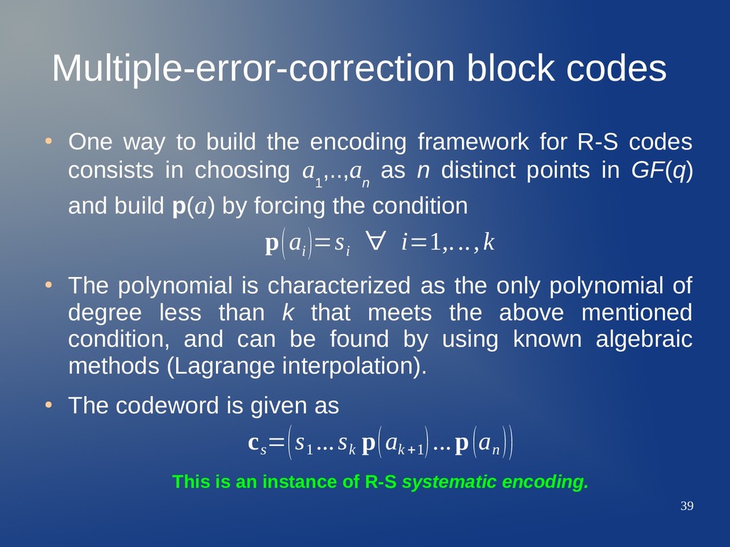
encoding framework for R-S codes consists in choosing a 1 ,..,a n as n distinct points in GF(q) and build p(a) by forcing the condition • The polynomial is characterized as the only polynomial of degree less than k that meets the above mentioned condition, and can be found by using known algebraic methods (Lagrange interpolation). • The codeword is given as This is an instance of R-S systematic encoding. p(a i )=s i ∀ i=1,...,k c s =(s 1 ...s k p(a k +1 )...p(a n ))
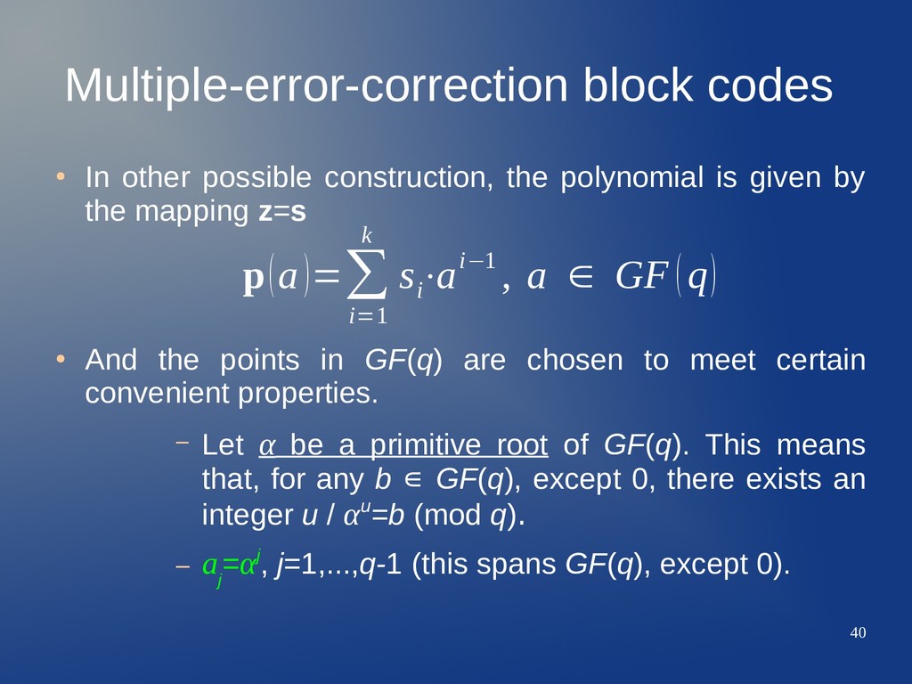
polynomial is given by the mapping z=s • And the points in GF(q) are chosen to meet certain convenient properties. – Let α be a primitive root of GF(q). This means that, for any b ∊ there iGF(q), except 0, there exists an integer u / αu=b (mod q). – a j =αj, j=1,...,q-1 there i(this spans GF(q), except 0). p(a)=∑ i=1 k s i ⋅ai−1 , a ∈ GF (q)
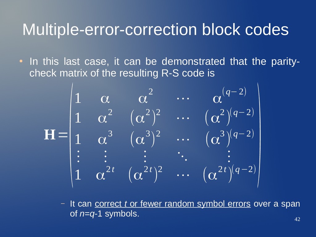
can be demonstrated that the parity- check matrix of the resulting R-S code is – It can correct t or fewer random symbol errors over a span of n=q-1 symbols. H= (1 α α2 ⋯ α(q−2) 1 α2 (α2 )2 ⋯ (α2 )(q−2) 1 α3 (α3 )2 ⋯ (α3 )(q−2) ⋮ ⋮ ⋮ ⋱ ⋮ 1 α2t (α2t )2 ⋯ (α2t )(q−2) )
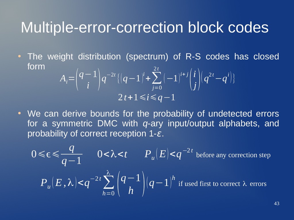
R-S codes has closed form • We can derive bounds for the probability of undetected errors for a symmetric DMC with q-ary input/output alphabets, and probability of correct reception 1-ε. A i =(q−1 i )q−2t {(q−1)i +∑ j=0 2t (−1)i+ j(i j )(q2t −qi)} 2t+1⩽i⩽q−1 P u (E)<q−2t before any correction step P u (E,λ)<q−2t ∑ h=0 λ (q−1 h )(q−1)h if used first to correct λ errors 0⩽ϵ⩽ q q−1 0<λ<t
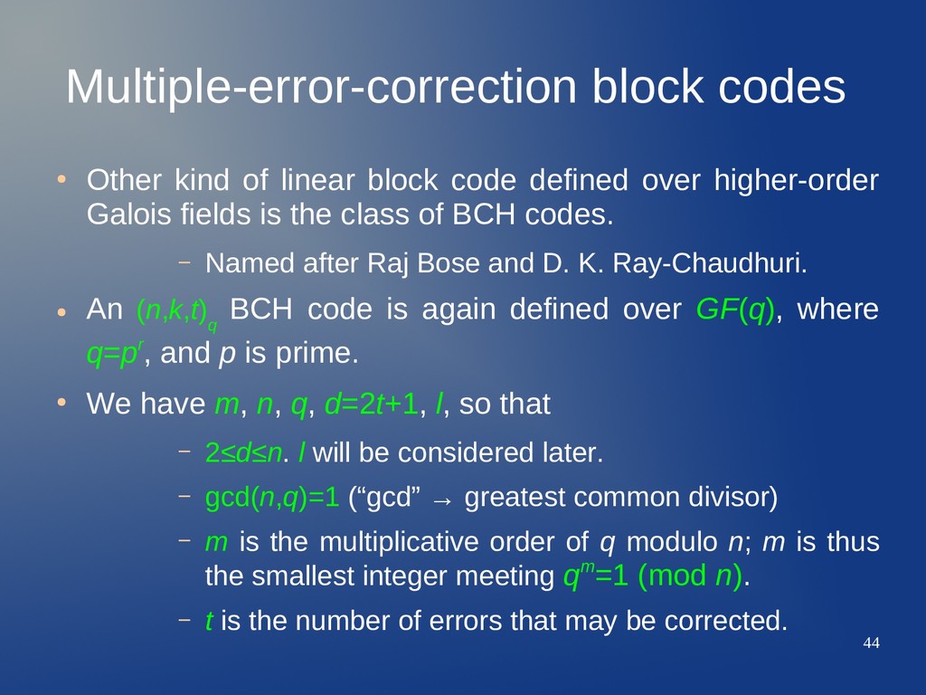
code defined over higher-order Galois fields is the class of BCH codes. – Named after Raj Bose and D. K. Ray-Chaudhuri. • An (n,k,t) q BCH code is again defined over GF(q), where q=pr, and p is prime. • We have m, n, q, d=2t+1, l, so that – 2≤d≤n. l will be considered later. – gcd(n,q)=1 (“gcd” → greatest common divisor) – m is the multiplicative order of q modulo n; m is thus the smallest integer meeting qm=1 (mod n). – t is the number of errors that may be corrected.
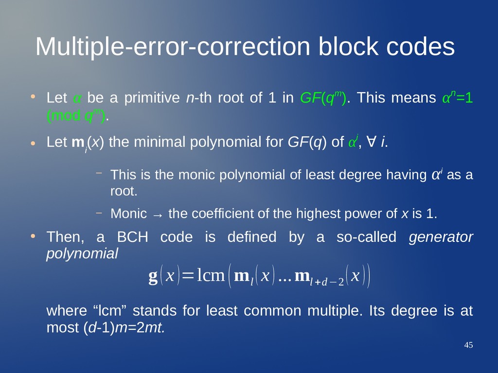
n-th root of 1 in GF(qm). This means αn=1 (mod qm). • Let m i (x) the minimal polynomial for GF(q) of αi, ∀ i. – This is the monic polynomial of least degree having αi as a root. – Monic → the coefficient of the highest power of x is 1. • Then, a BCH code is defined by a so-called generator polynomial where “lcm” stands for least common multiple. Its degree is at most (d-1)m=2mt. g(x)=lcm(m l (x)...m l+d−2 (x))
polynomial is done by building a polynomial containing the information symbols • Then there i there i there i there i there i there i there i there i there i there i there i there i there i there i there i there i there i there i • We may do systematic encoding as s (x)=∑ i=1 k s i ⋅xi−1 s=(s 1 ...s k ) ∈ GF (q)k → c(x)=∑ i=1 n c i ⋅xi−1 =s(x)⋅g (x), c i ∈ GF(q) → c=(c 1 ...c n ) c s (x)=xn−k ⋅s(x) ⏟ systematic symbols +xn−k ⋅s (x) mod g(x) ⏟ redundancy symbols
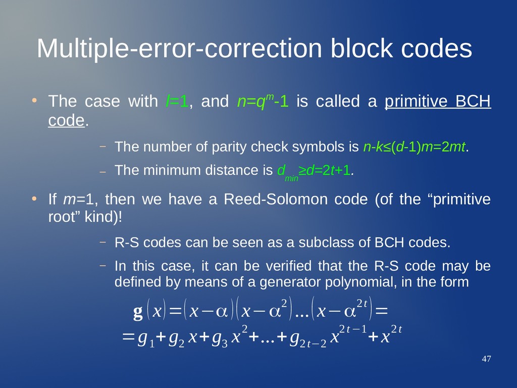
n=qm-1 is called a primitive BCH code. – The number of parity check symbols is n-k≤(d-1)m=2mt. – The minimum distance is d min ≥d=2t+1. • If m=1, then we have a Reed-Solomon code (of the “primitive root” kind)! – R-S codes can be seen as a subclass of BCH codes. – In this case, it can be verified that the R-S code may be defined by means of a generator polynomial, in the form g (x)=(x−α)(x−α2)...(x−α2t)= =g 1 +g 2 x+g 3 x2 +...+g 2t−2 x2t−1 +x2t
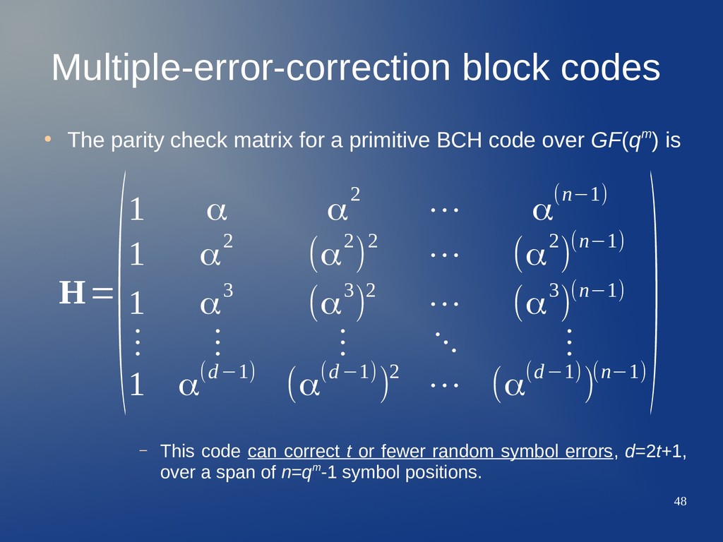
a primitive BCH code over GF(qm) is – This code can correct t or fewer random symbol errors, d=2t+1, over a span of n=qm-1 symbol positions. H= (1 α α2 ⋯ α(n−1) 1 α2 (α2 )2 ⋯ (α2 )(n−1) 1 α3 (α3 )2 ⋯ (α3 )(n−1) ⋮ ⋮ ⋮ ⋱ ⋮ 1 α(d−1) (α(d−1))2 ⋯ (α(d−1))(n−1) )
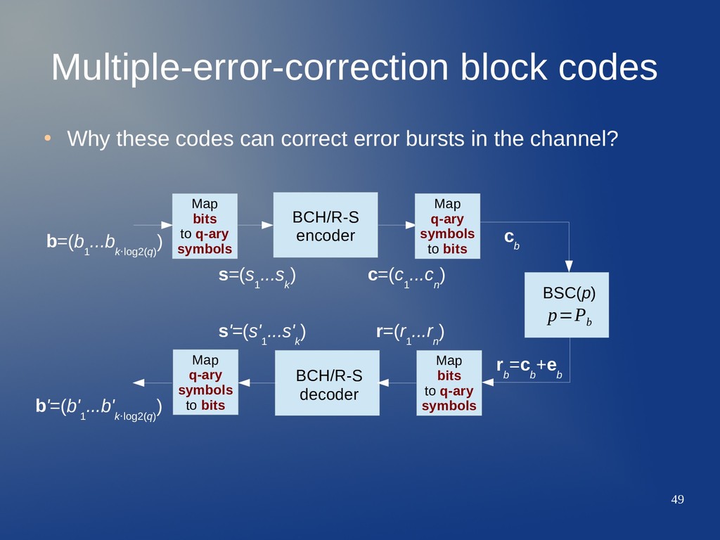
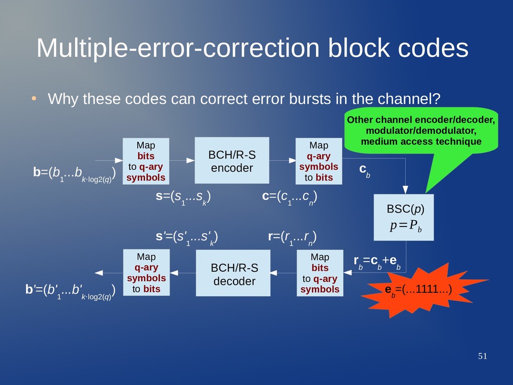
error bursts in the channel? BCH/R-S encoder BSC(p) BCH/R-S decoder Map bits to q-ary symbols Map q-ary symbols to bits Map q-ary symbols to bits Map bits to q-ary symbols s=(s 1 ...s k ) r=(r 1 ...r n ) b=(b 1 ...b k·log2(q) ) b'=(b' 1 ...b' k·log2(q) ) s'=(s' 1 ...s' k ) c=(c 1 ...c n ) c b r b =c b +e b p=P b
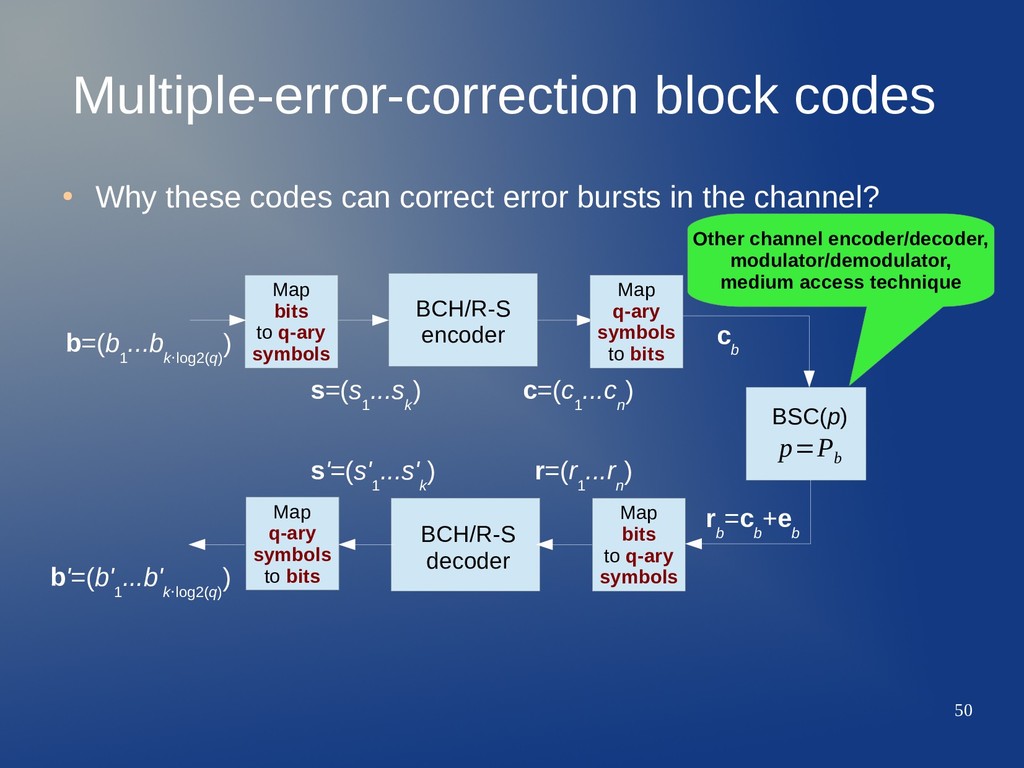
error bursts in the channel? BCH/R-S encoder BSC(p) BCH/R-S decoder Map bits to q-ary symbols Map q-ary symbols to bits Map q-ary symbols to bits Map bits to q-ary symbols s=(s 1 ...s k ) r=(r 1 ...r n ) b=(b 1 ...b k·log2(q) ) b'=(b' 1 ...b' k·log2(q) ) s'=(s' 1 ...s' k ) c=(c 1 ...c n ) Other channel encoder/decoder, modulator/demodulator, medium access technique c b r b =c b +e b p=P b
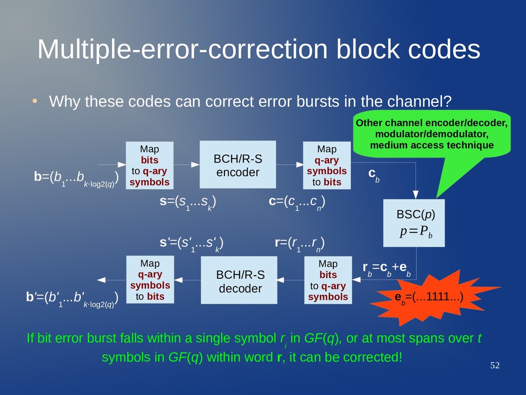
error bursts in the channel? BCH/R-S encoder BSC(p) BCH/R-S decoder Map bits to q-ary symbols Map q-ary symbols to bits Map q-ary symbols to bits Map bits to q-ary symbols e b =(...1111...) s=(s 1 ...s k ) r=(r 1 ...r n ) b=(b 1 ...b k·log2(q) ) b'=(b' 1 ...b' k·log2(q) ) s'=(s' 1 ...s' k ) c=(c 1 ...c n ) Other channel encoder/decoder, modulator/demodulator, medium access technique c b r b =c b +e b p=P b
error bursts in the channel? BCH/R-S encoder BSC(p) BCH/R-S decoder Map bits to q-ary symbols Map q-ary symbols to bits Map q-ary symbols to bits Map bits to q-ary symbols e b =(...1111...) s=(s 1 ...s k ) r=(r 1 ...r n ) b=(b 1 ...b k·log2(q) ) b'=(b' 1 ...b' k·log2(q) ) s'=(s' 1 ...s' k ) c=(c 1 ...c n ) Other channel encoder/decoder, modulator/demodulator, medium access technique If bit error burst falls within a single symbol r i in GF(q), or at most spans over t symbols in GF(q) within word r, it can be corrected! c b r b =c b +e b p=P b
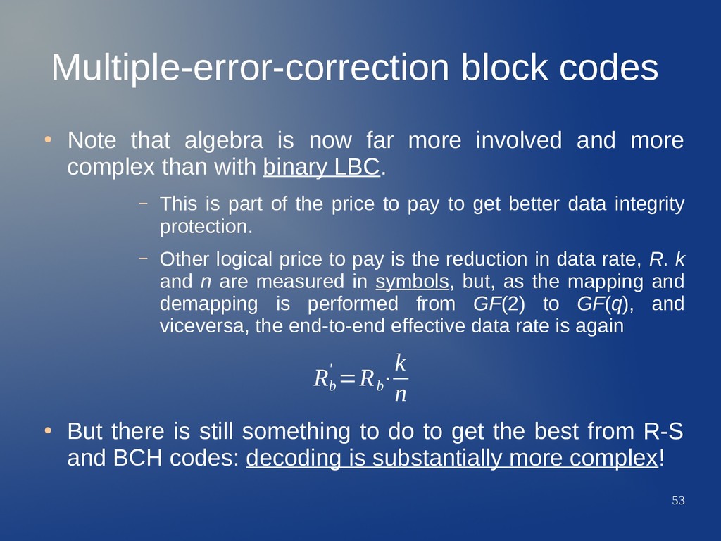
far more involved and more complex than with binary LBC. – This is part of the price to pay to get better data integrity protection. – Other logical price to pay is the reduction in data rate, R. k and n are measured in symbols, but, as the mapping and demapping is performed from GF(2) to GF(q), and viceversa, the end-to-end effective data rate is again • But there is still something to do to get the best from R-S and BCH codes: decoding is substantially more complex! R b ' =R b ⋅ k n
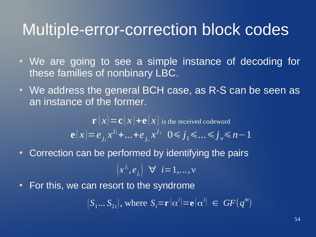
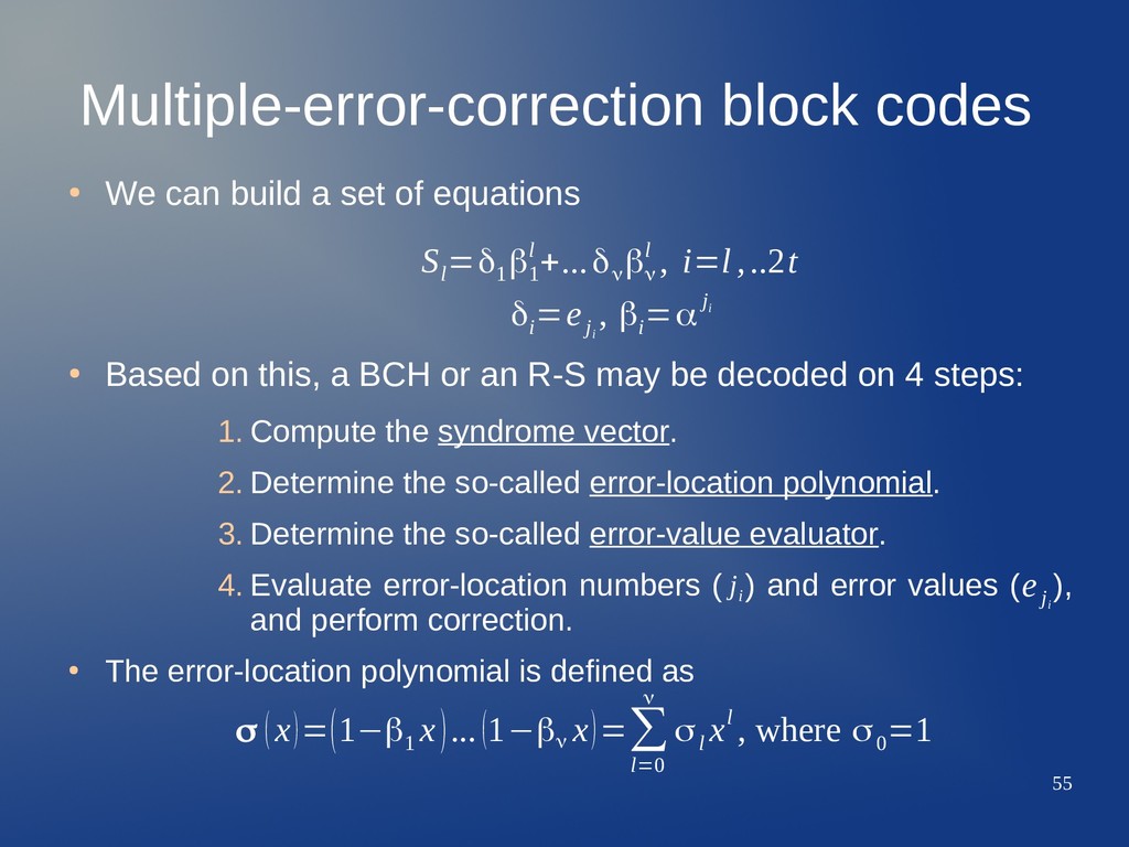
a simple instance of decoding for these families of nonbinary LBC. • We address the general BCH case, as R-S can be seen as an instance of the former. • Correction can be performed by identifying the pairs • For this, we can resort to the syndrome r (x)=c(x)+e(x) is the received codeword e(x)=e j 1 xj 1 +...+e j ν xj ν 0⩽ j 1 ⩽...⩽j ν ⩽n−1 (x j i ,e j i ) ∀ i=1,...,ν (S 1 ... S 2t ), where S i =r (αi)=e(αi) ∈ GF(qm )
ν β ν l , i=l ,..2t δi =e j i , βi =αj i • We can build a set of equations • Based on this, a BCH or an R-S may be decoded on 4 steps: 1. Compute the syndrome vector. 2. Determine the so-called error-location polynomial. 3. Determine the so-called error-value evaluator. 4. Evaluate error-location numbers ( ) and error values ( ), and perform correction. • The error-location polynomial is defined as j i e j i σ (x)=(1−β1 x)...(1−βν x)=∑ l=0 ν σl xl , where σ0 =1
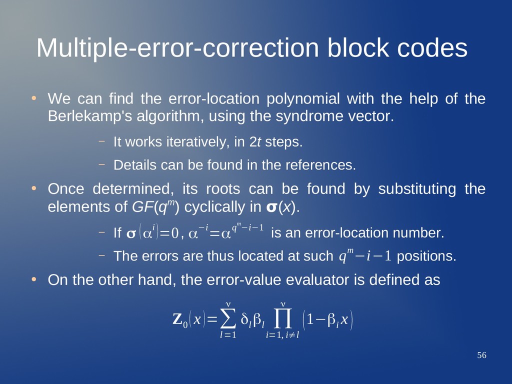
polynomial with the help of the Berlekamp's algorithm, using the syndrome vector. – It works iteratively, in 2t steps. – Details can be found in the references. • Once determined, its roots can be found by substituting the elements of GF(qm) cyclically in σ(x). – If , is an error-location number. – The errors are thus located at such positions. • On the other hand, the error-value evaluator is defined as σ (αi)=0 α−i =αqm −i−1 qm −i−1 Z 0 (x)=∑ l=1 ν δl βl ∏ i=1, i≠l ν (1−βi x)
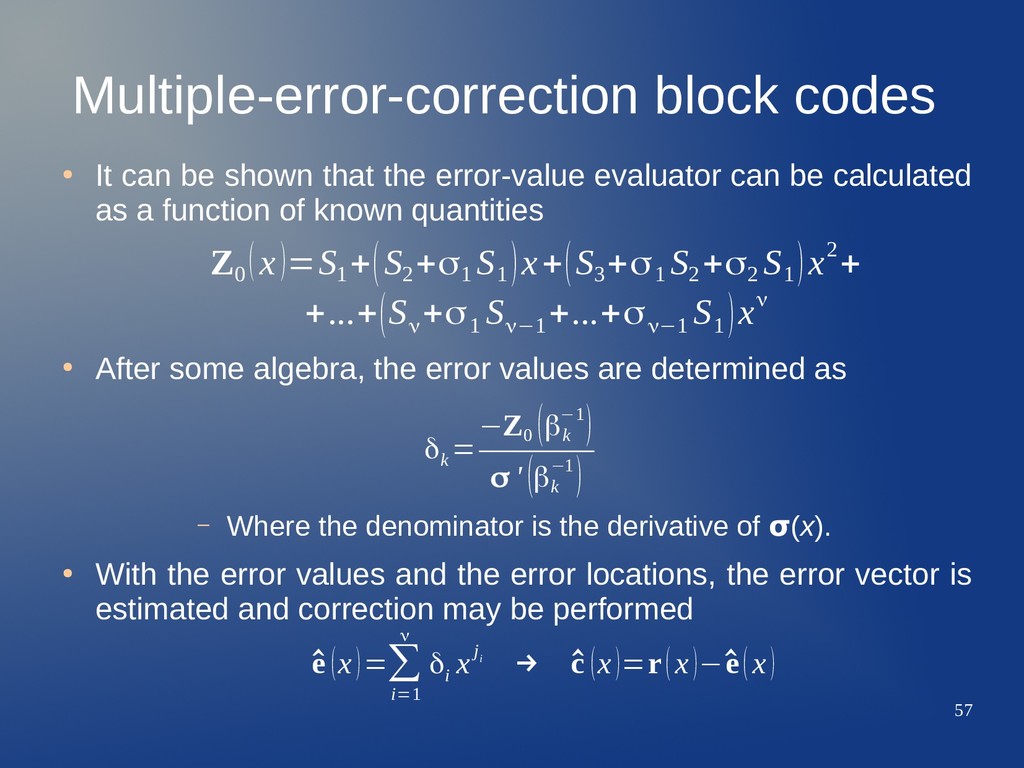
the error-value evaluator can be calculated as a function of known quantities • After some algebra, the error values are determined as – Where the denominator is the derivative of σ(x). • With the error values and the error locations, the error vector is estimated and correction may be performed Z 0 (x)=S 1 +(S 2 +σ1 S 1 )x+(S 3 +σ1 S 2 +σ2 S 1 )x2 + +...+(S ν +σ1 S ν−1 +...+σ ν−1 S 1 )xν δk = −Z 0 (βk −1) σ ' (βk −1) ^ e (x)=∑ i=1 ν δi xj i → ^ c (x)=r(x)−^ e(x)
be very powerful, but the amount of algebra required is very high. – The supporting theory is very complex, and designing and analyzing these codes require mastering algebra and geometry over finite-size fields. – All the operations are to be understood in GF(q) or GF(qm), when corresponding. • Nonbinary LBC of the kind described are usually employed in sophisticated FEC strategies for specific channels. – Binary LBC are more usual in ARQ strategies.
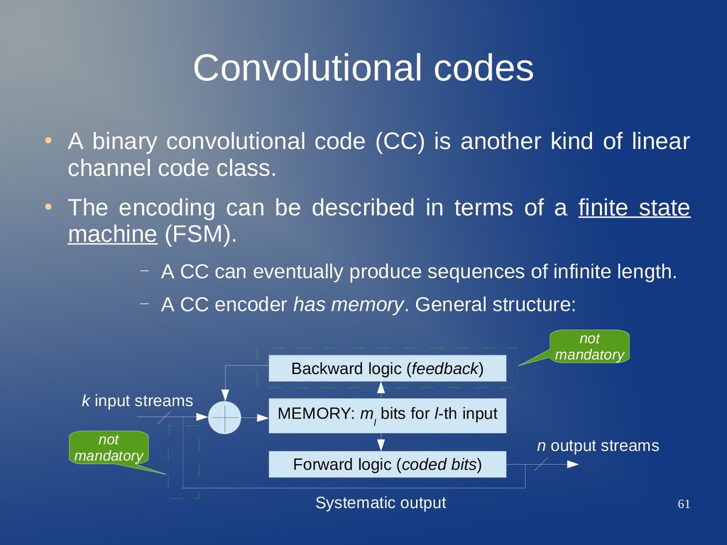
another kind of linear channel code class. • The encoding can be described in terms of a finite state machine (FSM). – A CC can eventually produce sequences of infinite length. – A CC encoder has memory. General structure: MEMORY: m l bits for l-th input Forward logic (coded bits) Backward logic (feedback) k input streams n output streams not mandatory not mandatory Systematic output
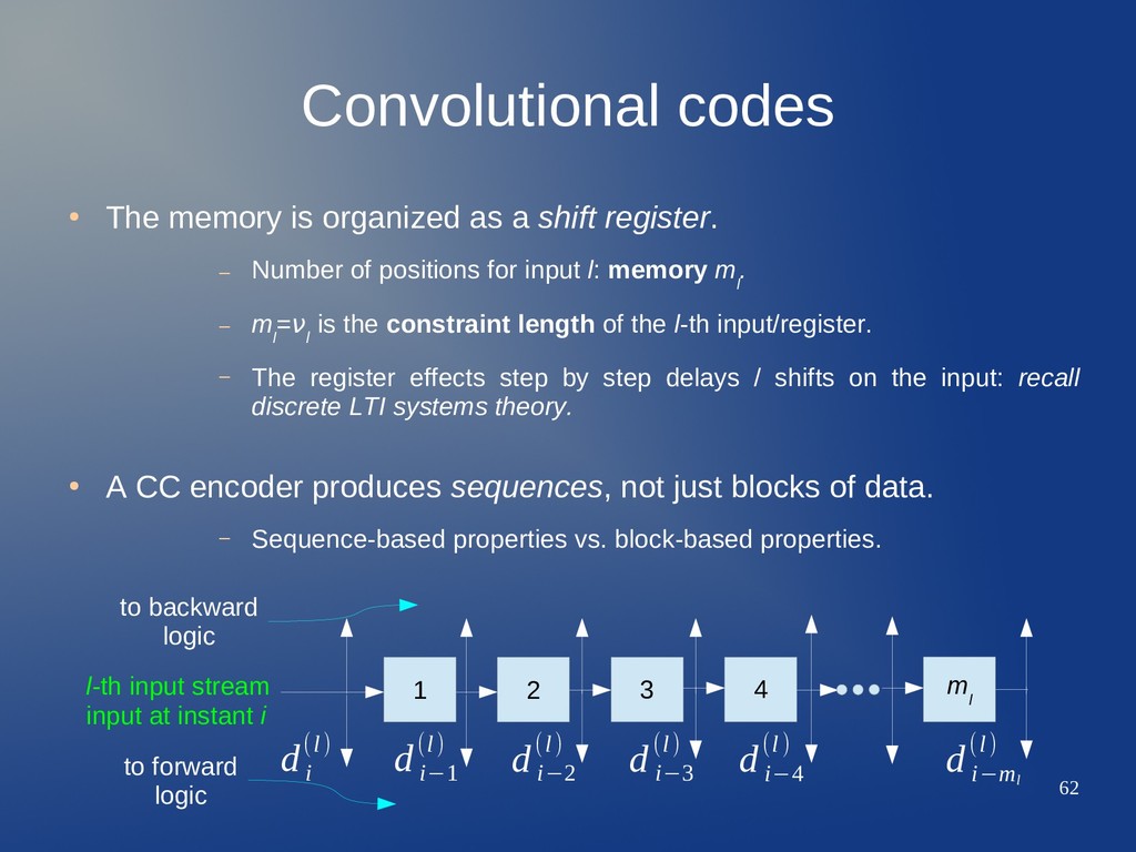
shift register. – Number of positions for input l: memory m l . – m l =ν l is the constraint length of the l-th input/register. – The register effects step by step delays / shifts on the input: recall discrete LTI systems theory. • A CC encoder produces sequences, not just blocks of data. – Sequence-based properties vs. block-based properties. 1 2 3 4 m l l-th input stream input at instant i to backward logic to forward logic d i (l) d i−1 (l) d i−2 (l) d i−3 (l) d i−4 (l) d i−m l (l)
boolean logic. – Very easy: each operation adds up (XOR) a number of memory positions, from each of the k inputs. • , is 1 when the p-th register position for the l- th input is added to get the j-th output. c i ( j)=∑ l=1 k ∑ q=i i−m l g l , q−i ( j) ⋅d q (l) j-th output at instant i inputs from all the k registers at instant i g l , p ( j) , p=0,... , m l Same structure for backward logic
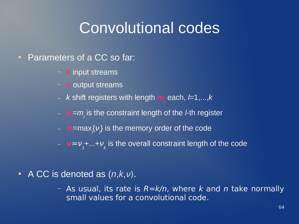
– k input streams – n output streams – k shift registers with length m l each, l=1,...,k – ν l =m l is the constraint length of the l-th register – m=max l {ν l } is the memory order of the code – ν=ν 1 +...+ν k is the overall constraint length of the code • A CC is denoted as (n,k,ν). – As there iusual, there iits there irate there iis there iR=k/n, there iwhere there ik there iand there in there itake there inormally there i small there ivalues there ifor there ia there iconvolutional there icode.
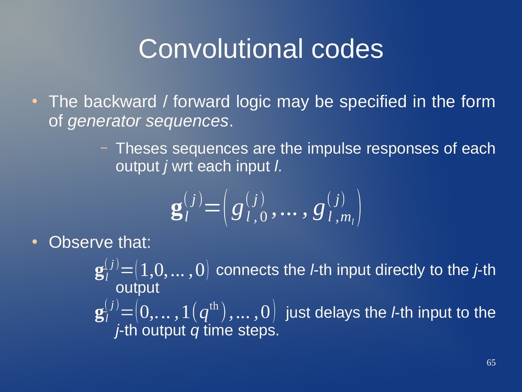
be specified in the form of generator sequences. – Theses sequences are the impulse responses of each output j wrt each input l. • Observe that: – connects the l-th input directly to the j-th output – just delays the l-th input to the j-th output q time steps. g l ( j)=(g l , 0 ( j) ,... , g l ,m l ( j) ) g l ( j)=(1,0,... ,0) g l ( j)=(0,... ,1(qth),... ,0)
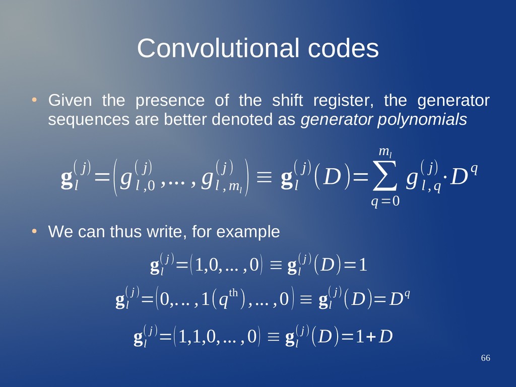
register, the generator sequences are better denoted as generator polynomials • We can thus write, for example g l ( j)=(g l ,0 ( j) ,... , g l , m l ( j) )≡ g l ( j)(D)=∑ q=0 m l g l, q ( j)⋅Dq g l ( j)=(1,0,... ,0) ≡ g l ( j)(D)=1 g l ( j)=(0,... ,1(qth),... ,0) ≡ g l ( j)(D)=Dq g l ( j)=(1,1,0,... ,0) ≡ g l ( j)(D)=1+D
a binary CC is linear and the sequences produced constitute CC codewords. • A feedforward CC (without backward logic - feedback) can be denoted in matrix from as G(D)= (g 1 (1)(D) g 1 (2)(D) ⋯ g 1 (n)(D) g 2 (1)(D) g 2 (2)(D) ⋯ g 2 (n)(D) ⋮ ⋮ ⋱ ⋮ g k (1)(D) g k (2)(D) ⋯ g k (n)(D) )
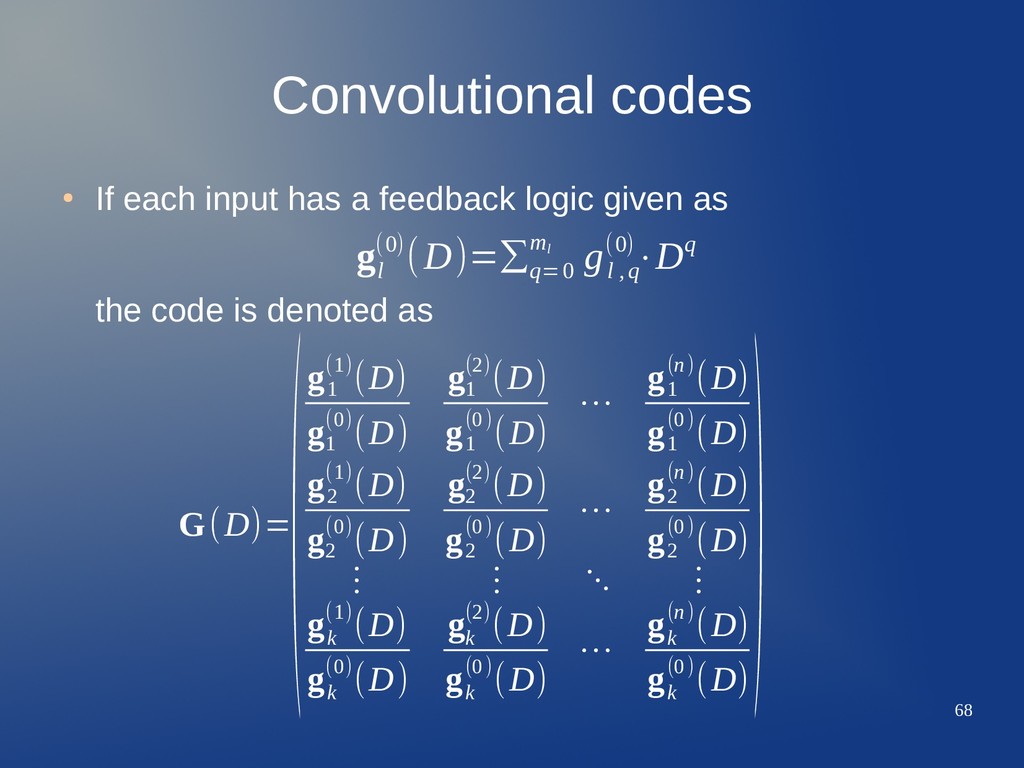
logic given as the code is denoted as g l (0)(D)=∑q=0 m l g l , q (0)⋅Dq G(D)= (g 1 (1)(D) g 1 (0)(D) g 1 (2)(D) g 1 (0)(D) ⋯ g 1 (n)(D) g 1 (0)(D) g 2 (1)(D) g 2 (0)(D) g 2 (2)(D) g 2 (0)(D) ⋯ g 2 (n)(D) g 2 (0)(D) ⋮ ⋮ ⋱ ⋮ g k (1)(D) g k (0)(D) g k (2)(D) g k (0)(D) ⋯ g k (n)(D) g k (0)(D) )
parity-check matrix H(D). – An (n,k,ν) CC is fully specified by G(D) or H(D). • Based on the matrix description, there are a good deal linear tools for design, analysis and evaluation of a given CC. • A regular CC can be described as a (canonical) all-feedforward CC and through an equivalent feedback (recursive) CC. – Note that a recursive CC can be seen as an IIR filter in GF(2). • Even though k and n could be very small, a CC has a very rich algebraic structure. – This has to do with the constraint length of the CC. – Each output bit is related to the present and past inputs via powerful algebraic methods.
classified as: – Systematic and feedforward (NSC). – Systematic and recursive (RSC). – Non-systematic and feedforward. – Non-systematic and recursive. • RSC is a popular class of CC, because it may provide an infinite output for a finite-weight input (IIR behavior). • Each NSC can be converted straightforwardly to a RSC with similar error correcting properties. • CC encoders are easy to implement with standard hardware: shift registers + combinational logic.
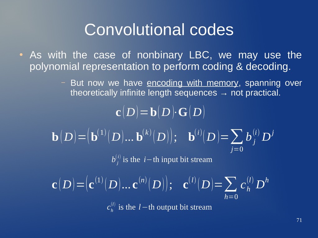
LBC, we may use the polynomial representation to perform coding & decoding. – But now we have encoding with memory, spanning over theoretically infinite length sequences → not practical. c(D)=b(D )⋅G(D) b(D)=(b(1) (D)... b(k) (D)); b(i)(D )=∑ j=0 b j (i) Dj b j (i) is the i−th input bit stream c(D)=(c(1) (D)...c(n) (D)); c(l) (D)=∑ h=0 c h (l) Dh c h (l) is the l−th output bit stream
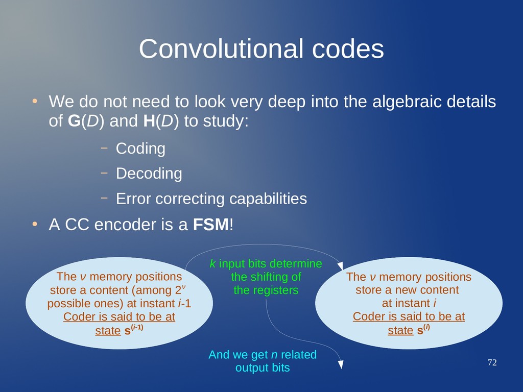
very deep into the algebraic details of G(D) and H(D) to study: – Coding – Decoding – Error correcting capabilities • A CC encoder is a FSM! The ν memory positions store a content (among 2ν possible ones) at instant i-1 Coder is said to be at state s(i-1) The ν memory positions store a new content at instant i Coder is said to be at state s(i) k input bits determine the shifting of the registers And we get n related output bits
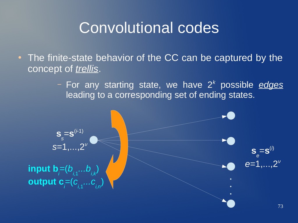
can be captured by the concept of trellis. – For any starting state, we have 2k possible edges leading to a corresponding set of ending states. s s =s(i-1) s=1,...,2ν s e =s(i) e=1,...,2ν input b i =(b i,1 ...b i,k ) output c i =(c i,1 ...c i,n )
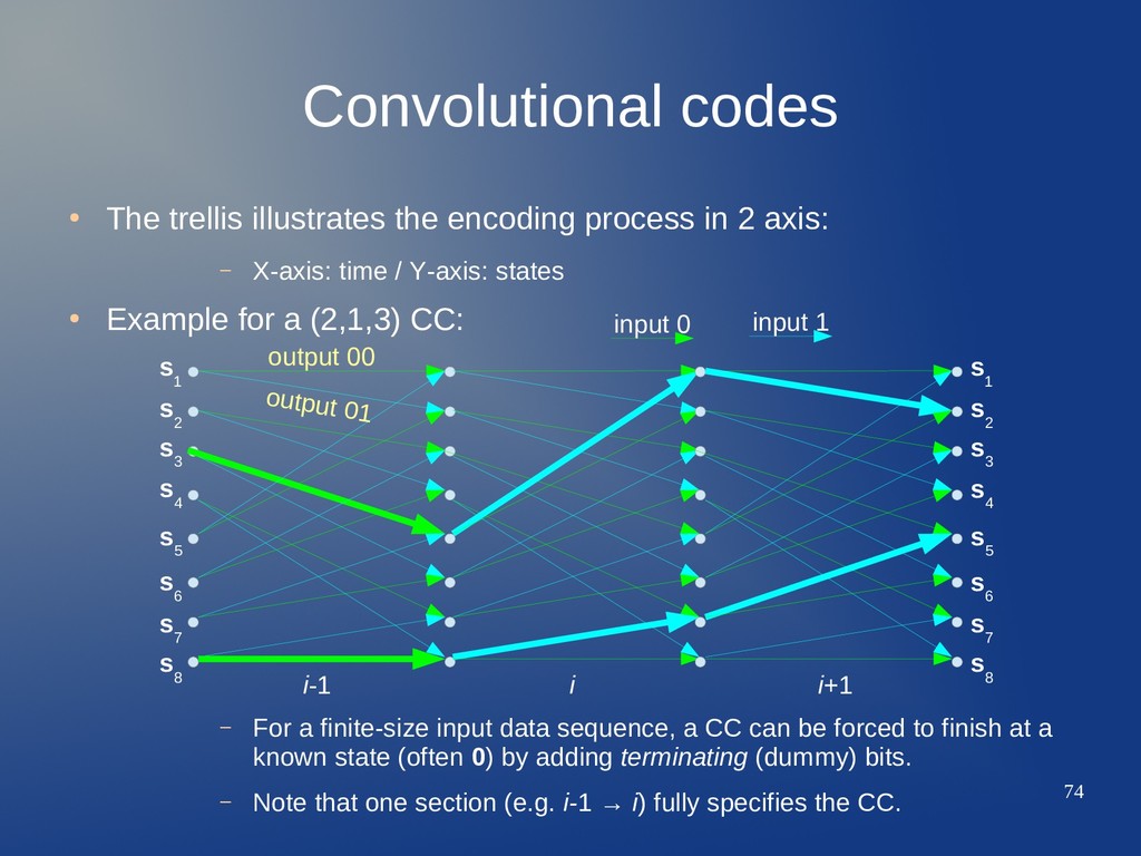
in 2 axis: – X-axis: time / Y-axis: states • Example for a (2,1,3) CC: – For a finite-size input data sequence, a CC can be forced to finish at a known state (often 0) by adding terminating (dummy) bits. – Note that one section (e.g. i-1 → i) fully specifies the CC. output 00 output 01 s 2 s 1 s 3 s 4 s 6 s 5 s 7 s 8 s 2 s 3 s 4 s 6 s 5 s 7 s 8 s 1 i-1 i i+1 input 0 input 1
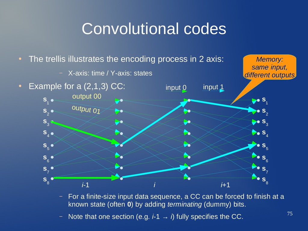
in 2 axis: – X-axis: time / Y-axis: states • Example for a (2,1,3) CC: – For a finite-size input data sequence, a CC can be forced to finish at a known state (often 0) by adding terminating (dummy) bits. – Note that one section (e.g. i-1 → i) fully specifies the CC. output 00 output 01 s 2 s 1 s 3 s 4 s 6 s 5 s 7 s 8 s 2 s 3 s 4 s 6 s 5 s 7 s 8 s 1 i-1 i i+1 input 0 input 1 Memory: Memory: same input, same input, different outputs different outputs
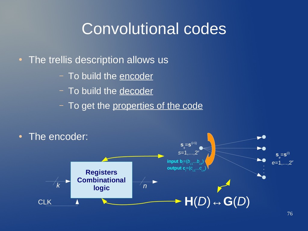
To build the encoder – To build the decoder – To get the properties of the code • The encoder: H(D)↔G(D) Registers Combinational logic k n CLK s s =s(i-1) s=1,...,2ν s e =s(i) e=1,...,2ν input b i =(b i,1 ...b i,k ) output c i =(c i,1 ...c i,n )
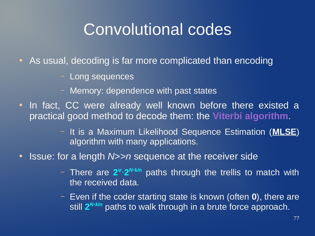
complicated than encoding – Long sequences – Memory: dependence with past states • In fact, CC were already well known before there existed a practical good method to decode them: the Viterbi algorithm. – It is a Maximum Likelihood Sequence Estimation (MLSE) algorithm with many applications. • Issue: for a length N>>n sequence at the receiver side – There are 2ν·2N·k/n paths through the trellis to match with the received data. – Even if the coder starting state is known (often 0), there are still 2N·k/n paths to walk through in a brute force approach.
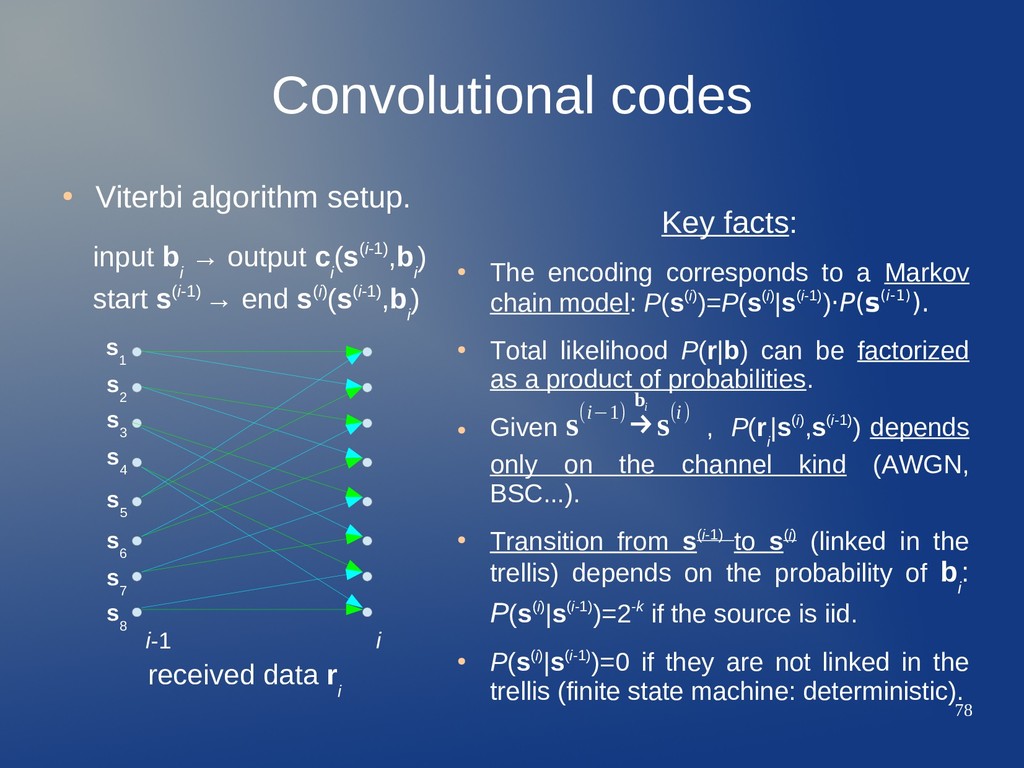
3 s 4 s 6 s 5 s 7 s 8 s 1 i-1 i input b i → output c i (s(i-1),b i ) start s(i-1) → end s(i)(s(i-1),b i ) received data r i Key facts: • The encoding corresponds to a Markov chain model: P(s(i))=P(s(i)|s(i-1))·P(s(i-1)). • Total likelihood P(r|b) can be factorized as a product of probabilities. • Given , P(r i |s(i),s(i-1)) depends only on the channel kind (AWGN, BSC...). • Transition from s(i-1) to s(i) (linked in the trellis) depends on the probability of b i : P(s(i)|s(i-1))=2-k if the source is iid. • P(s(i)|s(i-1))=0 if they are not linked in the trellis (finite state machine: deterministic). s(i−1)→ b i s(i)
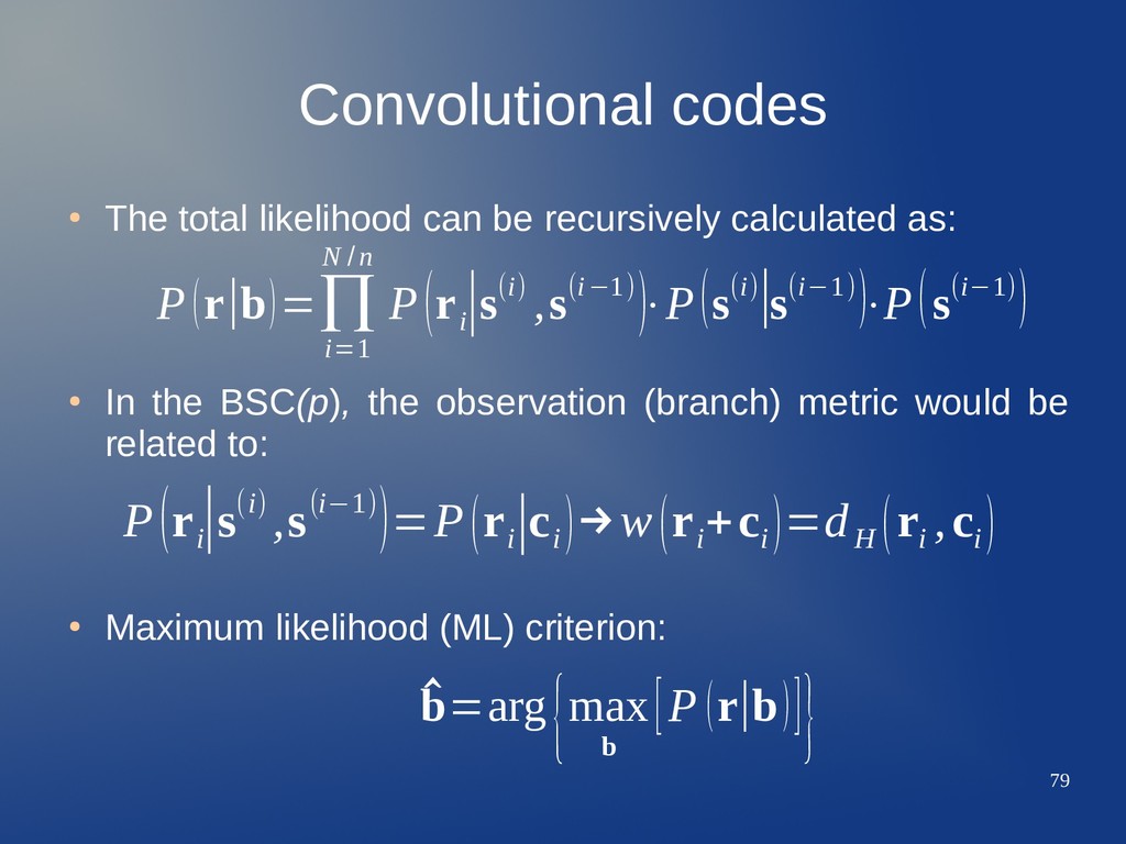
calculated as: • In the BSC(p), the observation (branch) metric would be related to: • Maximum likelihood (ML) criterion: P(r i |s(i) ,s(i−1))=P(r i |c i )→w (r i +c i )=d H (r i ,c i ) P(r∣b)=∏ i=1 N /n P(r i ∣s(i) ,s(i−1))⋅P(s(i)∣s(i−1))⋅P(s(i−1)) ̂ b=arg{max b [P (r∣b)]}
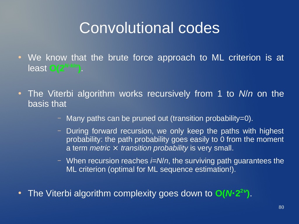
approach to ML criterion is at least O(2N·k/n). • The Viterbi algorithm works recursively from 1 to N/n on the basis that – Many paths can be pruned out (transition probability=0). – During forward recursion, we only keep the paths with highest probability: the path probability goes easily to 0 from the moment a term metric ⨯ transition probability is very small. – When recursion reaches i=N/n, the surviving path guarantees the ML criterion (optimal for ML sequence estimation!). • The Viterbi algorithm complexity goes down to O(N·22ν).
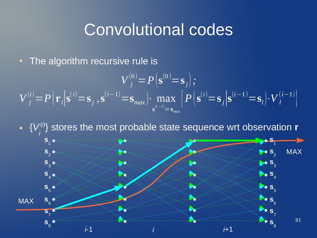
{V j (i)} stores the most probable state sequence wrt observation r V j (0)=P(s(0)=s j ); V j (i)=P(r i ∣s(i)=s j ,s(i−1)=s max )⋅ max s(i−1)=s max {P(s(i)=s j ∣s(i−1)=s l )⋅V l (i−1)} s 2 s 1 s 3 s 4 s 6 s 5 s 7 s 8 s 2 s 3 s 4 s 6 s 5 s 7 s 8 s 1 i-1 i i+1 MAX MAX
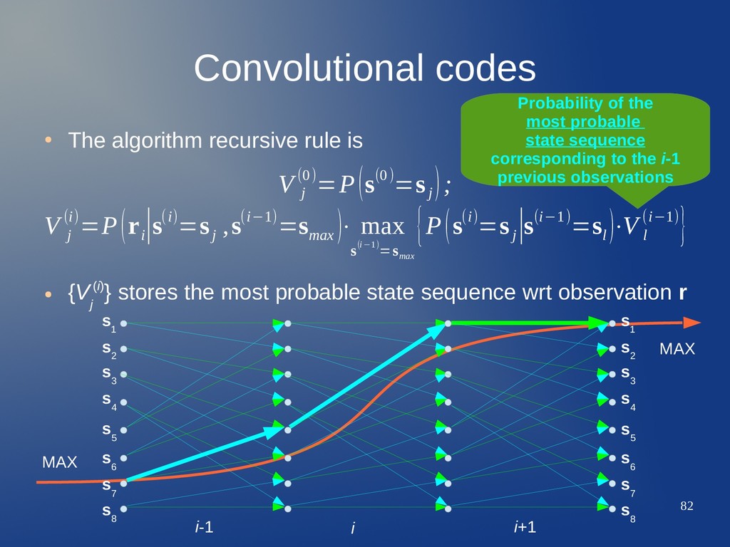
{V j (i)} stores the most probable state sequence wrt observation r V j (0)=P(s(0)=s j ); V j (i)=P(r i ∣s(i)=s j ,s(i−1)=s max )⋅ max s(i−1)=s max {P(s(i)=s j ∣s(i−1)=s l )⋅V l (i−1)} Probability of the most probable state sequence corresponding to the i-1 previous observations s 2 s 1 s 3 s 4 s 6 s 5 s 7 s 8 s 2 s 3 s 4 s 6 s 5 s 7 s 8 s 1 i-1 i i+1 MAX MAX
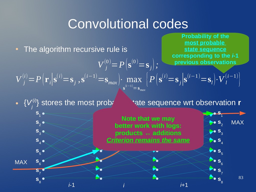
{V j (i)} stores the most probable state sequence wrt observation r V j (0)=P(s(0)=s j ); V j (i)=P(r i ∣s(i)=s j ,s(i−1)=s max )⋅ max s(i−1)=s max {P(s(i)=s j ∣s(i−1)=s l )⋅V l (i−1)} Probability of the most probable state sequence corresponding to the i-1 previous observations s 2 s 1 s 3 s 4 s 6 s 5 s 7 s 8 s 2 s 3 s 4 s 6 s 5 s 7 s 8 s 1 i-1 i i+1 MAX MAX Note that we may better work with logs: products ↔ additions Criterion remains the same
algorithm when the demodulator yields hard outputs – r i is a vector of n estimated bits (BSC(p) equivalent channel). • In AWGN, we can do better to decode a CC – We can provide soft (probabilistic) estimations for the observation metric. – For an iid source, we can easily get an observation transition metric based on the probability of each b i,l =0,1, l=1,...,k, associated to a possible transition. – There is a gain of around 2 dB in E b /N 0 . – LBC decoders can also accept soft inputs (non syndrome-based decoders). – We will examine an example of soft decoding of CC in the lab.
encoder and the decoder – Encoder: FSM (registers, combinational logic). – Decoder: Viterbi algorithm (for practical reasons, suboptimal adaptations are usually employed). • But what about performance? • First... – CC are mainly intended for FEC, not for ARQ schemes. – In a long sequence (=CC codeword), the probability of having at least one error is very high... – And... are we going to retransmit the whole sequence?
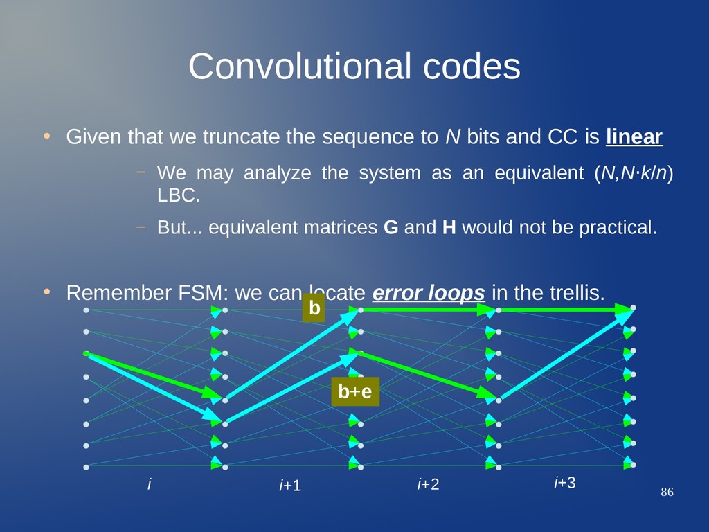
to N bits and CC is linear – We may analyze the system as an equivalent (N,N·k/n) LBC. – But... equivalent matrices G and H would not be practical. • Remember FSM: we can locate error loops in the trellis. i i+1 i+2 i+3 b b+e
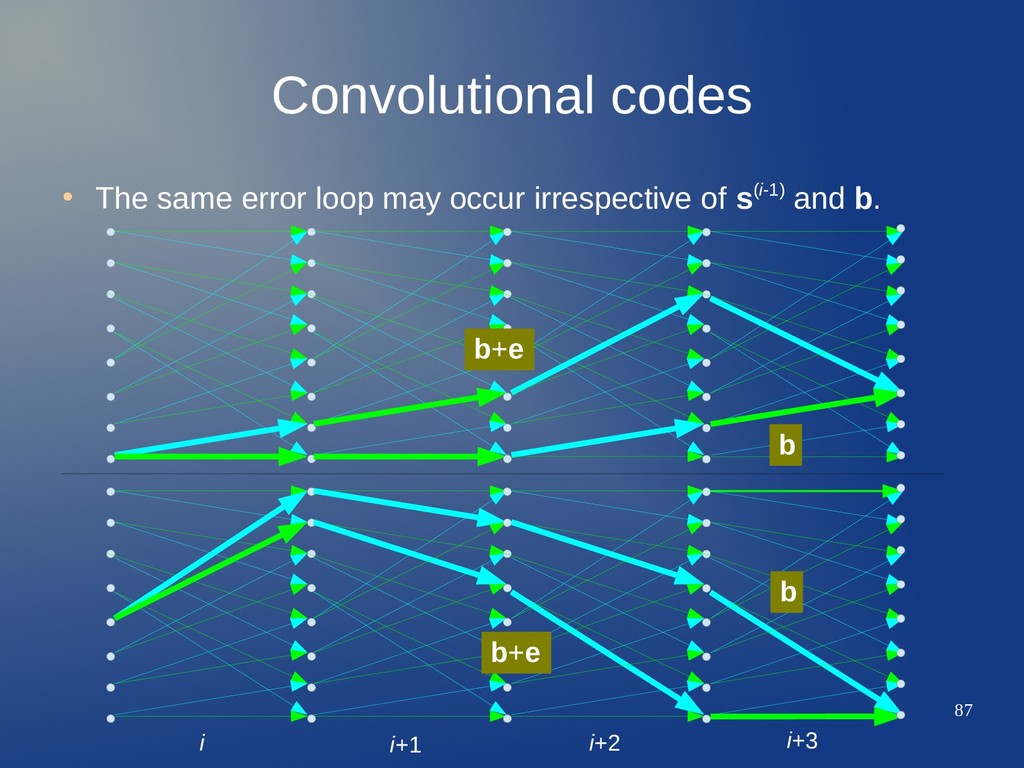
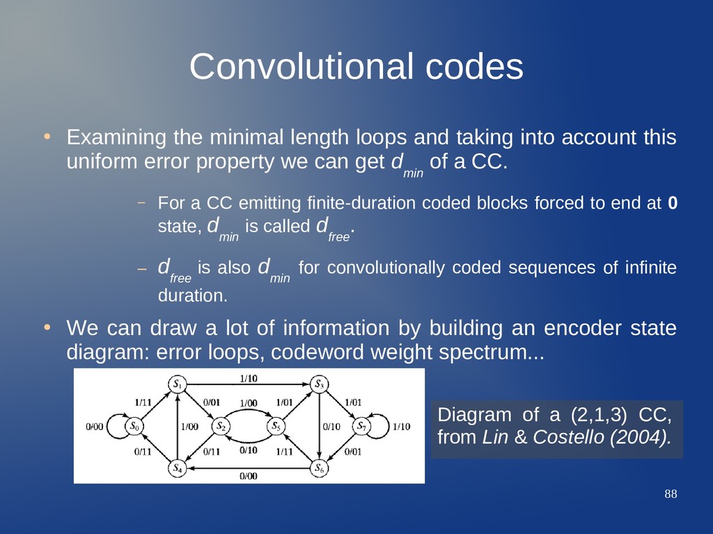
taking into account this uniform error property we can get d min of a CC. – For a CC emitting finite-duration coded blocks forced to end at 0 state, d min is called d free . – d free is also d min for convolutionally coded sequences of infinite duration. • We can draw a lot of information by building an encoder state diagram: error loops, codeword weight spectrum... Diagram of a (2,1,3) CC, from Lin & Costello (2004).
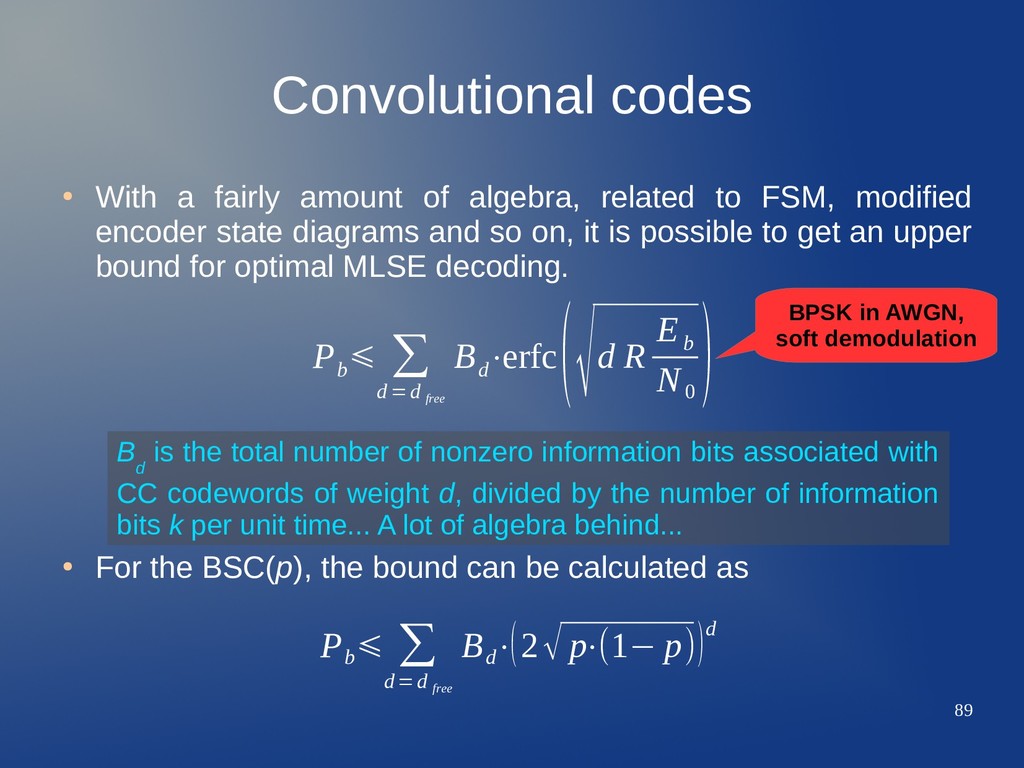
related to FSM, modified encoder state diagrams and so on, it is possible to get an upper bound for optimal MLSE decoding. • For the BSC(p), the bound can be calculated as P b ⩽ ∑ d=d free B d ⋅erfc (√d R E b N 0 ) B d is the total number of nonzero information bits associated with CC codewords of weight d, divided by the number of information bits k per unit time... A lot of algebra behind... BPSK in AWGN, soft demodulation P b ⩽ ∑ d= d free B d ⋅(2√ p⋅(1− p))d
decode a CC, and performance will vary accordingly. • A CC may be punctured to match other rates higher than R=k/n, but the resulting equivalent CC is clearly weaker. – Performance-rate trade-off. – Puncturing is a very usual tool that provides flexibility to the usage of CC's in practice. Native convolutional encoder k n Puncturing algorithm (prune bits) n'<n
Concatenated Convolutional Codes (PCCC). • Coding concatenation has been known and employed for decades, but TC added a joint efficient decoding algorithm. – Example of concatenated coding with independent decoding is the use of ARQ + FEC hybrid strategies (CRC/R-S + CC). CC 1 CC 2 ? k input streams n=n 1 +n 2 output streams Rate R=k/(n 1 +n 2 ) b c=c 1 ∪c 2
Concatenated Convolutional Codes (PCCC). • Coding concatenation has been known and employed for decades, but TC added a joint efficient decoding algorithm. – Example of concatenated coding with independent decoding is the use of ARQ + FEC hybrid strategies (CRC/R-S + CC). CC 1 CC 2 ? k input streams n=n 1 +n 2 output streams We will see this is a key element... Rate R=k/(n 1 +n 2 ) b c=c 1 ∪c 2
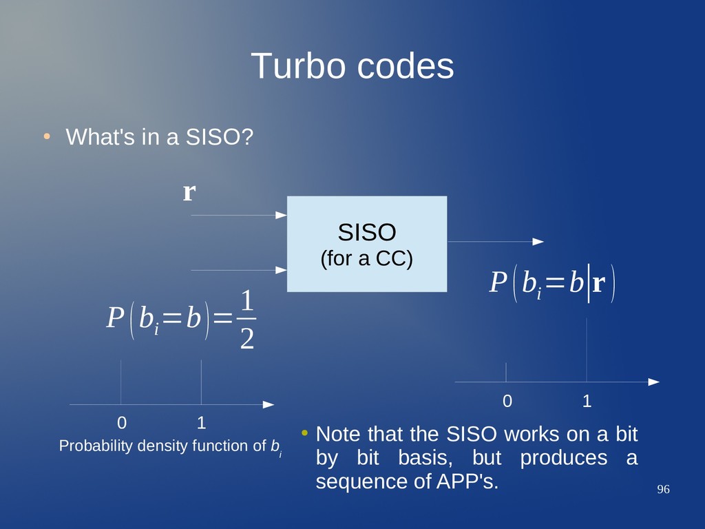
decoding with Viterbi algorithm relied on MLSE criterion. – This is optimal when binary data at CC input is iid. • For CC, we also have decoders that provide probabilistic (soft) outputs. – They convert a priori soft values + channel output soft estimations into updated a posteriori soft values. – They are optimal from the Maximum A Posteriori (MAP) criterion point of view. – They are called Soft Input-Soft Output (SISO) decoders.
a CC) 0 1 0 1 P(b i =b)= 1 2 P(b i =b∣r ) r • Note that the SISO works on a bit by bit basis, but produces a sequence of APP's. Probability density function of b i
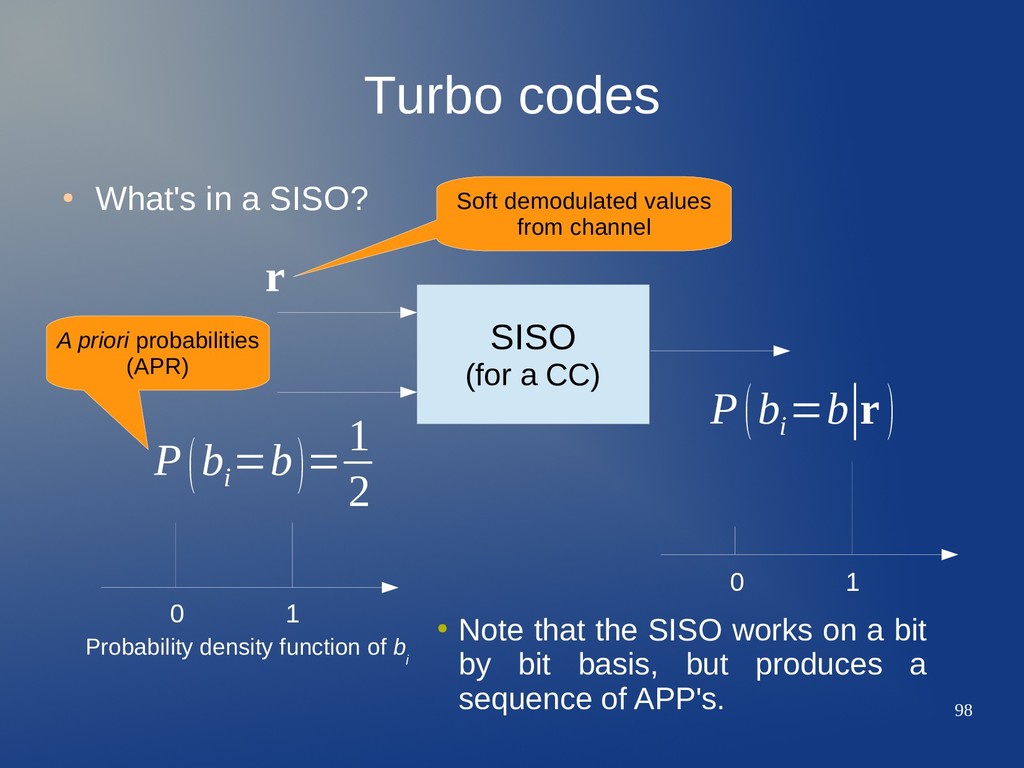
a CC) 0 1 0 1 P(b i =b)= 1 2 P(b i =b∣r ) r Soft demodulated values from channel • Note that the SISO works on a bit by bit basis, but produces a sequence of APP's. Probability density function of b i
a CC) 0 1 0 1 P(b i =b)= 1 2 P(b i =b∣r ) r Soft demodulated values from channel A priori probabilities (APR) • Note that the SISO works on a bit by bit basis, but produces a sequence of APP's. Probability density function of b i
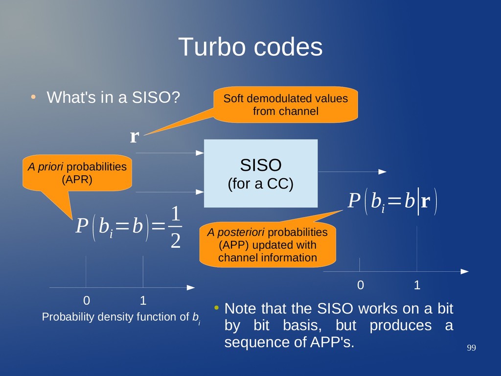
a CC) 0 1 0 1 P(b i =b)= 1 2 P(b i =b∣r ) r Soft demodulated values from channel A priori probabilities (APR) A posteriori probabilities (APP) updated with channel information • Note that the SISO works on a bit by bit basis, but produces a sequence of APP's. Probability density function of b i
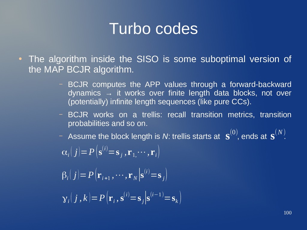
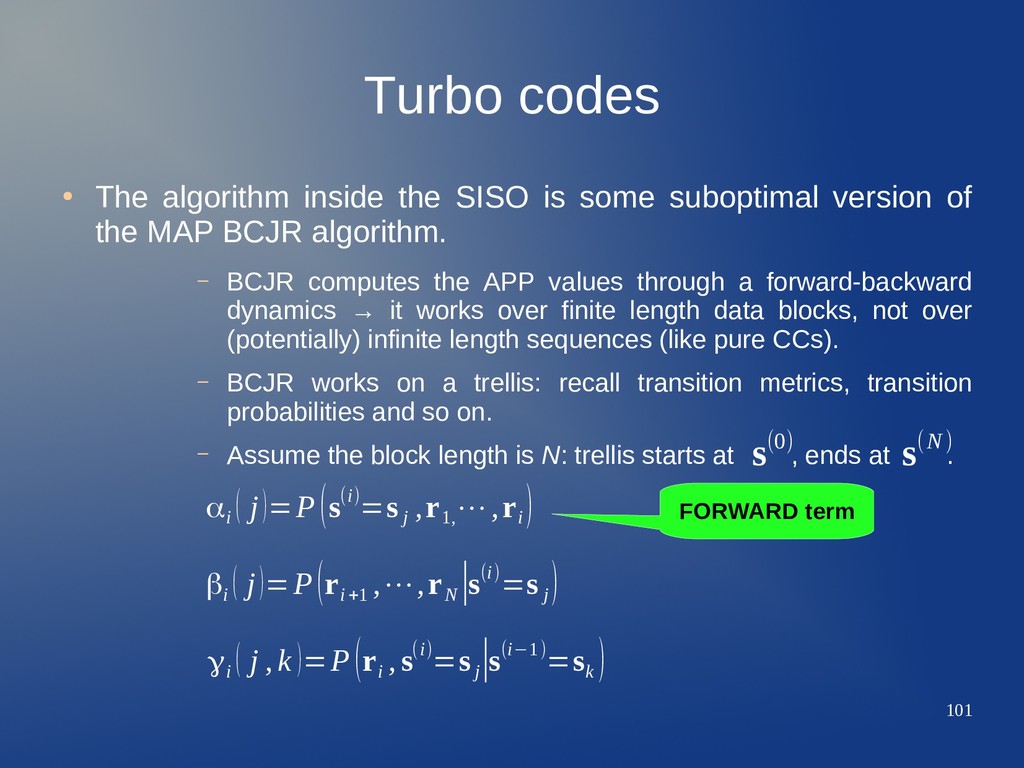
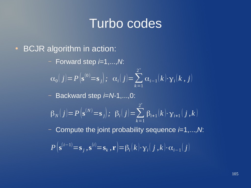
some suboptimal version of the MAP BCJR algorithm. – BCJR computes the APP values through a forward-backward dynamics → it works over finite length data blocks, not over (potentially) infinite length sequences (like pure CCs). – BCJR works on a trellis: recall transition metrics, transition probabilities and so on. – Assume the block length is N: trellis starts at , ends at . αi ( j)=P(s(i)=s j ,r 1, ⋯,r i ) βi ( j)=P(r i+1 ,⋯,r N ∣s(i)=s j ) γi ( j , k )=P(r i , s(i)=s j ∣s(i−1)=s k ) s(0) s(N )
some suboptimal version of the MAP BCJR algorithm. – BCJR computes the APP values through a forward-backward dynamics → it works over finite length data blocks, not over (potentially) infinite length sequences (like pure CCs). – BCJR works on a trellis: recall transition metrics, transition probabilities and so on. – Assume the block length is N: trellis starts at , ends at . αi ( j)=P(s(i)=s j ,r 1, ⋯,r i ) βi ( j)=P(r i+1 ,⋯,r N ∣s(i)=s j ) γi ( j , k )=P(r i , s(i)=s j ∣s(i−1)=s k ) FORWARD term s(0) s(N )
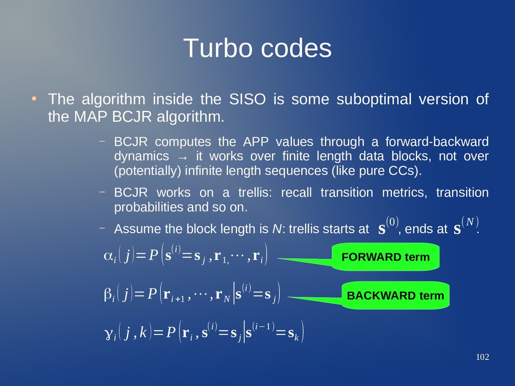
some suboptimal version of the MAP BCJR algorithm. – BCJR computes the APP values through a forward-backward dynamics → it works over finite length data blocks, not over (potentially) infinite length sequences (like pure CCs). – BCJR works on a trellis: recall transition metrics, transition probabilities and so on. – Assume the block length is N: trellis starts at , ends at . αi ( j)=P(s(i)=s j ,r 1, ⋯,r i ) βi ( j)=P(r i+1 ,⋯,r N ∣s(i)=s j ) γi ( j , k )=P(r i , s(i)=s j ∣s(i−1)=s k ) FORWARD term BACKWARD term s(0) s(N )
some suboptimal version of the MAP BCJR algorithm. – BCJR computes the APP values through a forward-backward dynamics → it works over finite length data blocks, not over (potentially) infinite length sequences (like pure CCs). – BCJR works on a trellis: recall transition metrics, transition probabilities and so on. – Assume the block length is N: trellis starts at , ends at . αi ( j)=P(s(i)=s j ,r 1, ⋯,r i ) βi ( j)=P(r i+1 ,⋯,r N ∣s(i)=s j ) γi ( j , k )=P(r i , s(i)=s j ∣s(i−1)=s k ) FORWARD term BACKWARD term TRANSITION s(0) s(N )
some suboptimal version of the MAP BCJR algorithm. – BCJR computes the APP values through a forward-backward dynamics → it works over finite length data blocks, not over (potentially) infinite length sequences (like pure CCs). – BCJR works on a trellis: recall transition metrics, transition probabilities and so on. – Assume the block length is N: trellis starts at , ends at . αi ( j)=P(s(i)=s j ,r 1, ⋯,r i ) βi ( j)=P(r i+1 ,⋯,r N ∣s(i)=s j ) γi ( j , k )=P(r i , s(i)=s j ∣s(i−1)=s k ) FORWARD term BACKWARD term TRANSITION s(0) s(N ) Remember, n components for an (n,k,ν) CC
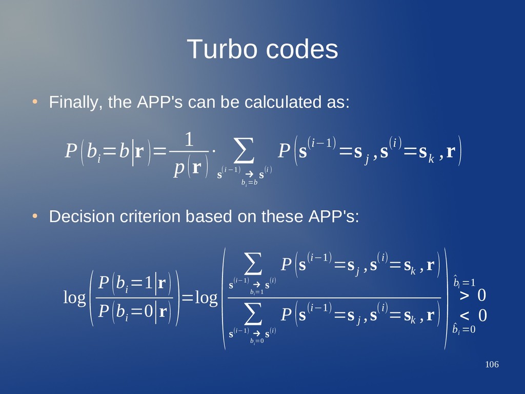
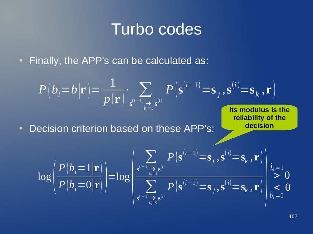
as: • Decision criterion based on these APP's: P(b i =b∣r )= 1 p(r ) ⋅ ∑ s(i−1) → b i =b s(i) P(s(i−1)=s j ,s(i)=s k ,r) log(P(b i =1|r) P(b i =0|r) )=log ( ∑ s(i−1) → b i =1 s(i) P(s(i−1)=s j ,s(i)=s k ,r) ∑ s(i−1) → b i =0 s(i) P(s(i−1)=s j ,s(i)=s k ,r) )> ^ b i =1 0 < ^ b i =0 0
as: • Decision criterion based on these APP's: P(b i =b∣r )= 1 p(r ) ⋅ ∑ s(i−1) → b i =b s(i) P(s(i−1)=s j ,s(i)=s k ,r) log(P(b i =1|r) P(b i =0|r) )=log ( ∑ s(i−1) → b i =1 s(i) P(s(i−1)=s j ,s(i)=s k ,r) ∑ s(i−1) → b i =0 s(i) P(s(i−1)=s j ,s(i)=s k ,r) )> ^ b i =1 0 < ^ b i =0 0 Its modulus is the reliability of the decision
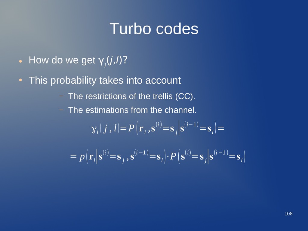
(j,l)? • This probability takes into account – The restrictions of the trellis (CC). – The estimations from the channel. γi ( j , l)=P(r i ,s(i)=s j ∣s(i−1)=s l )= = p(r i ∣s(i)=s j ,s(i−1)=s l )⋅P(s(i)=s j ∣s(i−1)=s l )
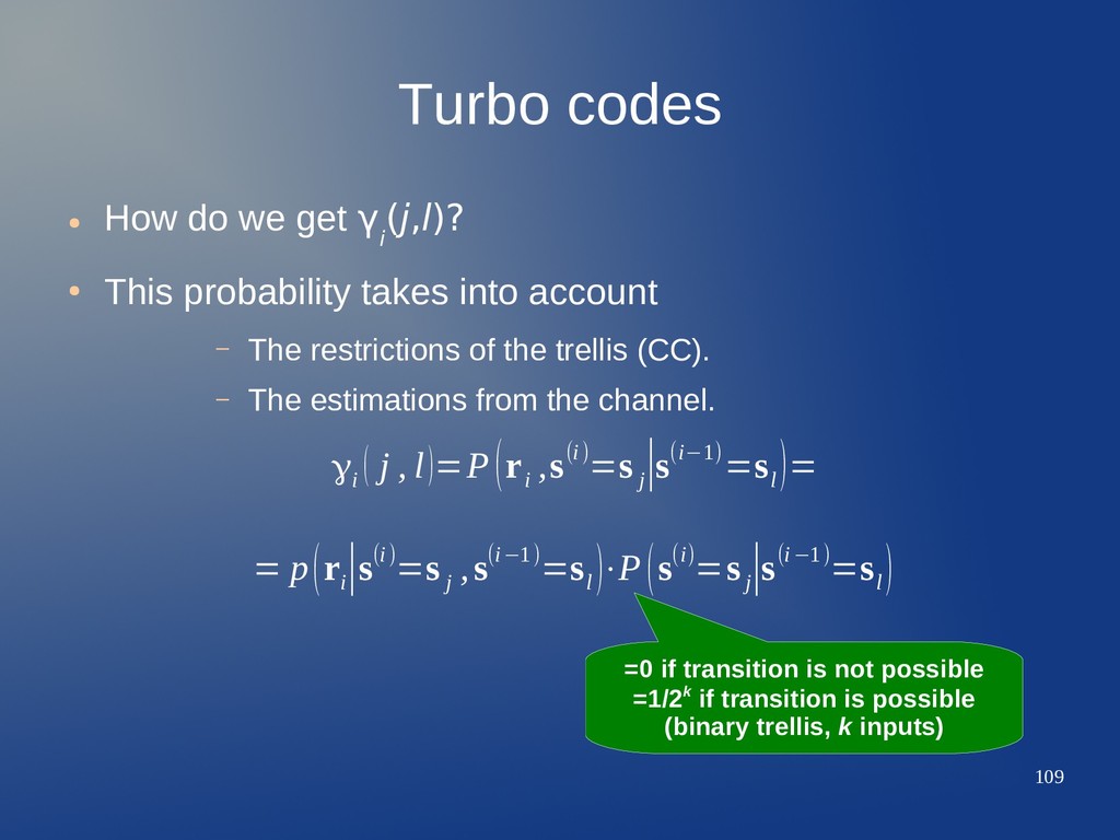
(j,l)? • This probability takes into account – The restrictions of the trellis (CC). – The estimations from the channel. γi ( j , l)=P(r i ,s(i)=s j ∣s(i−1)=s l )= = p(r i ∣s(i)=s j ,s(i−1)=s l )⋅P(s(i)=s j ∣s(i−1)=s l ) =0 if transition is not possible =1/2k if transition is possible (binary trellis, k inputs)
(j,l)? • This probability takes into account – The restrictions of the trellis (CC). – The estimations from the channel. γi ( j , l)=P(r i ,s(i)=s j ∣s(i−1)=s l )= = p(r i ∣s(i)=s j ,s(i−1)=s l )⋅P(s(i)=s j ∣s(i−1)=s l ) =0 if transition is not possible =1/2k if transition is possible (binary trellis, k inputs) in AWGN for unipolar c i,m 1 (2πσ2)n/2 ⋅e −∑ m =1 n (r i ,m −c i,m )2 2σ2
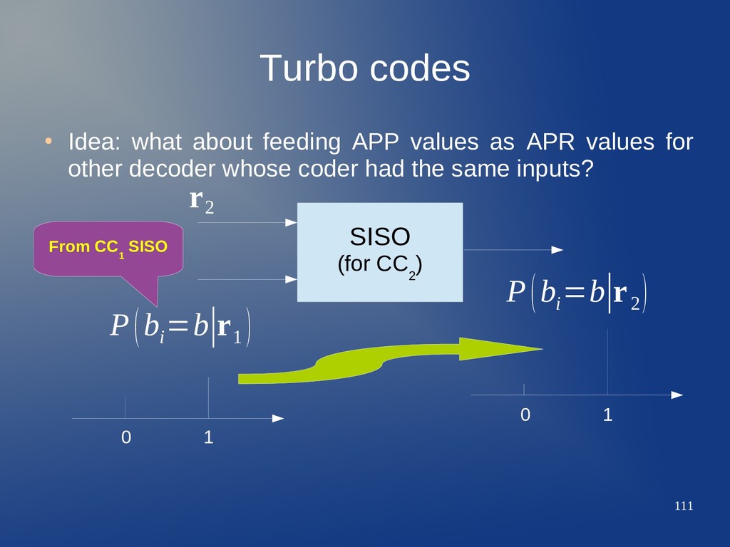
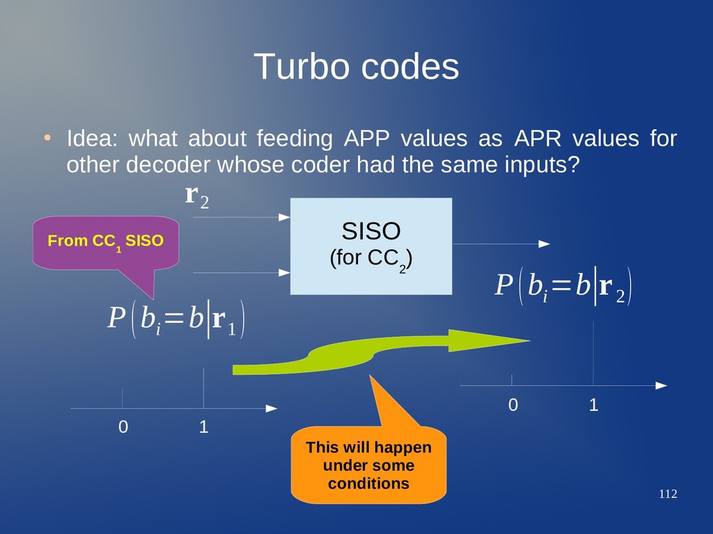
as APR values for other decoder whose coder had the same inputs? SISO (for CC 2 ) 0 1 0 1 P(b i =b∣r 1 ) P(b i =b∣r 2 ) r 2 From CC 1 SISO This will happen under some conditions
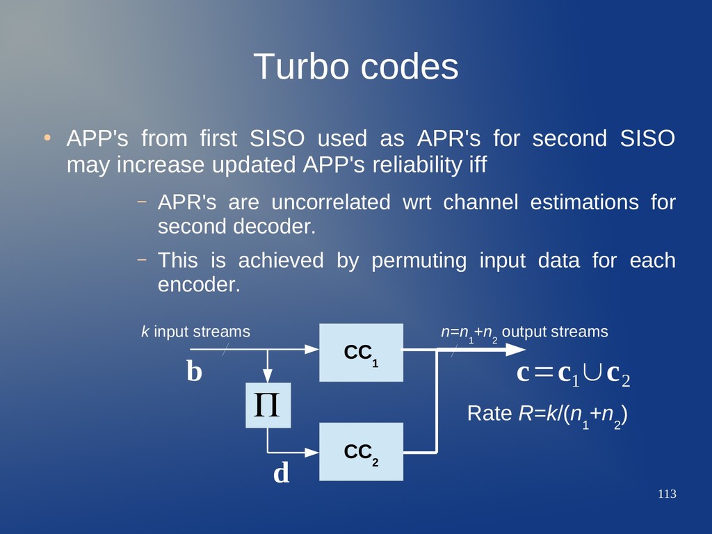
APR's for second SISO may increase updated APP's reliability iff – APR's are uncorrelated wrt channel estimations for second decoder. – This is achieved by permuting input data for each encoder. CC 1 CC 2 k input streams n=n 1 +n 2 output streams Rate R=k/(n 1 +n 2 ) b c=c 1 ∪c 2 Π d
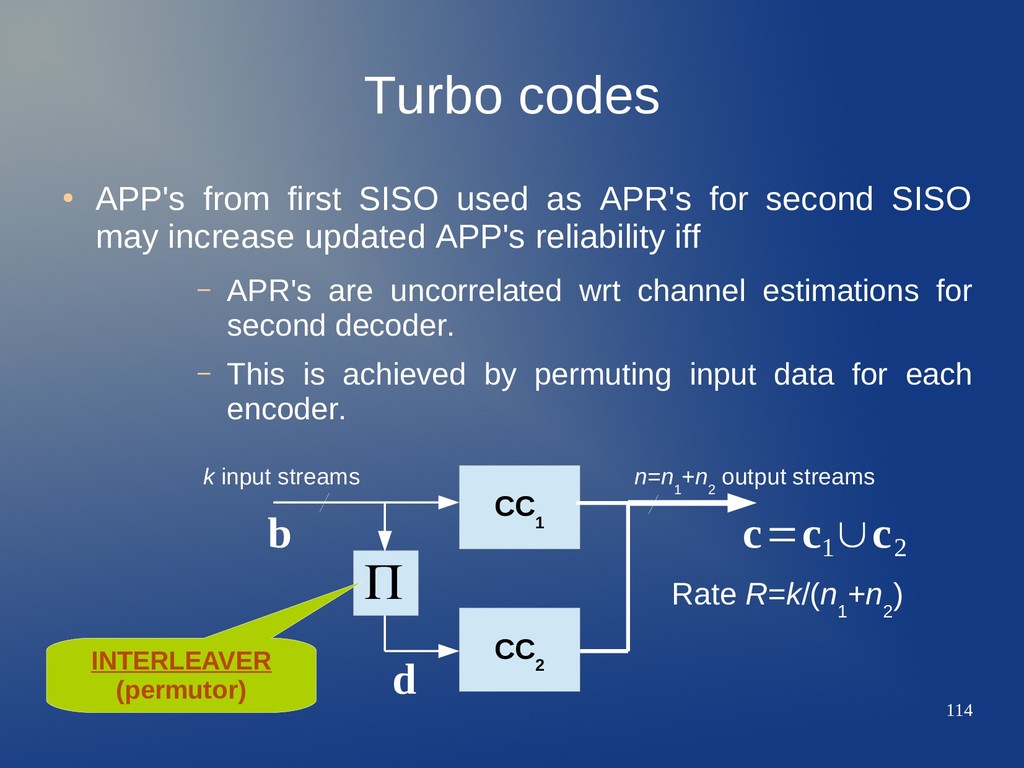
APR's for second SISO may increase updated APP's reliability iff – APR's are uncorrelated wrt channel estimations for second decoder. – This is achieved by permuting input data for each encoder. CC 1 CC 2 k input streams n=n 1 +n 2 output streams INTERLEAVER (permutor) Rate R=k/(n 1 +n 2 ) b c=c 1 ∪c 2 Π d
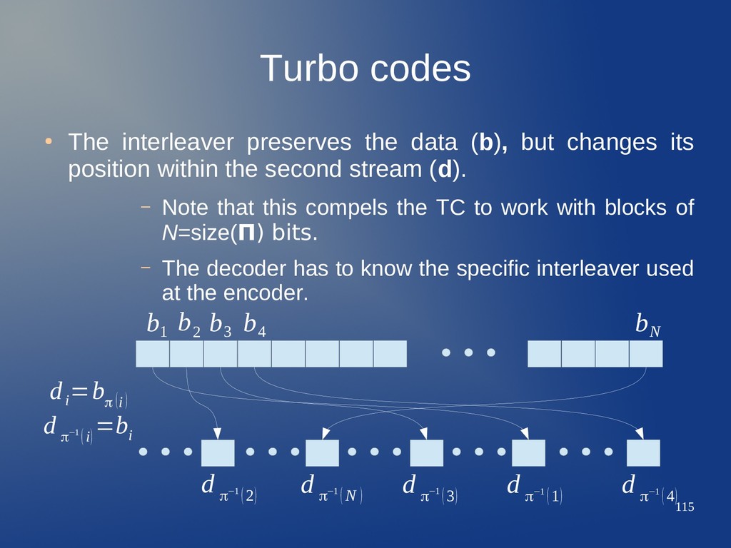
but changes its position within the second stream (d). – Note that this compels the TC to work with blocks of N=size(Π) there ibits. – The decoder has to know the specific interleaver used at the encoder. b 1 b 2 b 3 b 4 b N d π−1 (2) d π−1 (N ) d π−1 (3) d π−1 (1) d π−1 (4) d i =b π (i) d π−1 (i) =b i
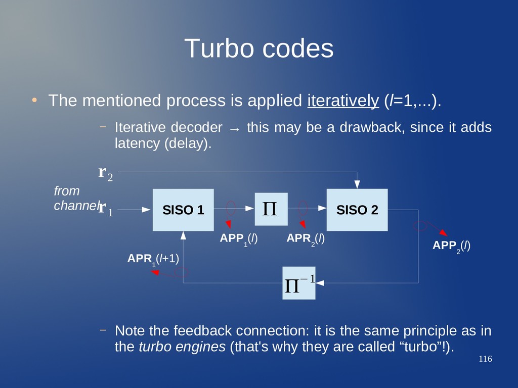
(l=1,...). – Iterative decoder → this may be a drawback, since it adds latency (delay). – Note the feedback connection: it is the same principle as in the turbo engines (that's why they are called “turbo”!). SISO 1 SISO 2 Π−1 Π r 2 r 1 APP 1 (l) APR 2 (l) APP 2 (l) APR 1 (l+1) from channel
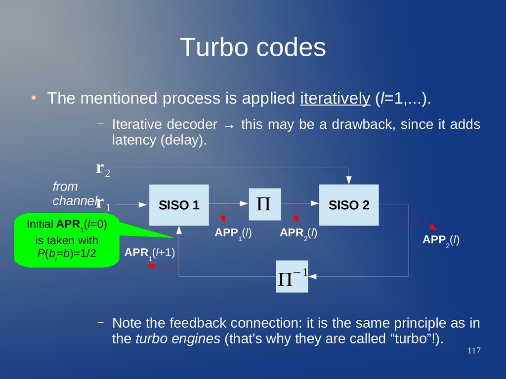
(l=1,...). – Iterative decoder → this may be a drawback, since it adds latency (delay). – Note the feedback connection: it is the same principle as in the turbo engines (that's why they are called “turbo”!). SISO 1 SISO 2 Π−1 Π r 2 r 1 APP 1 (l) APR 2 (l) APP 2 (l) APR 1 (l+1) from channel Initial APR 1 (l=0) is taken with P(b i =b)=1/2
log-probability values, that are in general denominated LLR in the literature (though they are strictly not so). • SISO 1 output LLR for i-th bit and l-th iteration can be factorized as – is the input APR value from previous SISO. – is the so-called extrinsic output value (only term interchanged). SISO 1 SISO 2 Π−1 Π r 2 r 1 L e1 (l) L a2 (l) L e2 (l) L a1 (l+1) from channel Π−1 decision L 1 i (l)=log (P(b i =1|r,l) P(b i =0|r,l) )=L a1 i (l)+L e 1 i (l) L e 1 i (l) L a1 i (l)
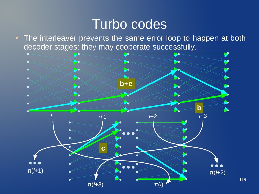
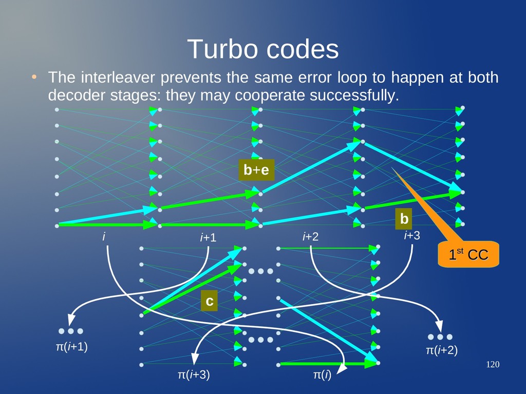
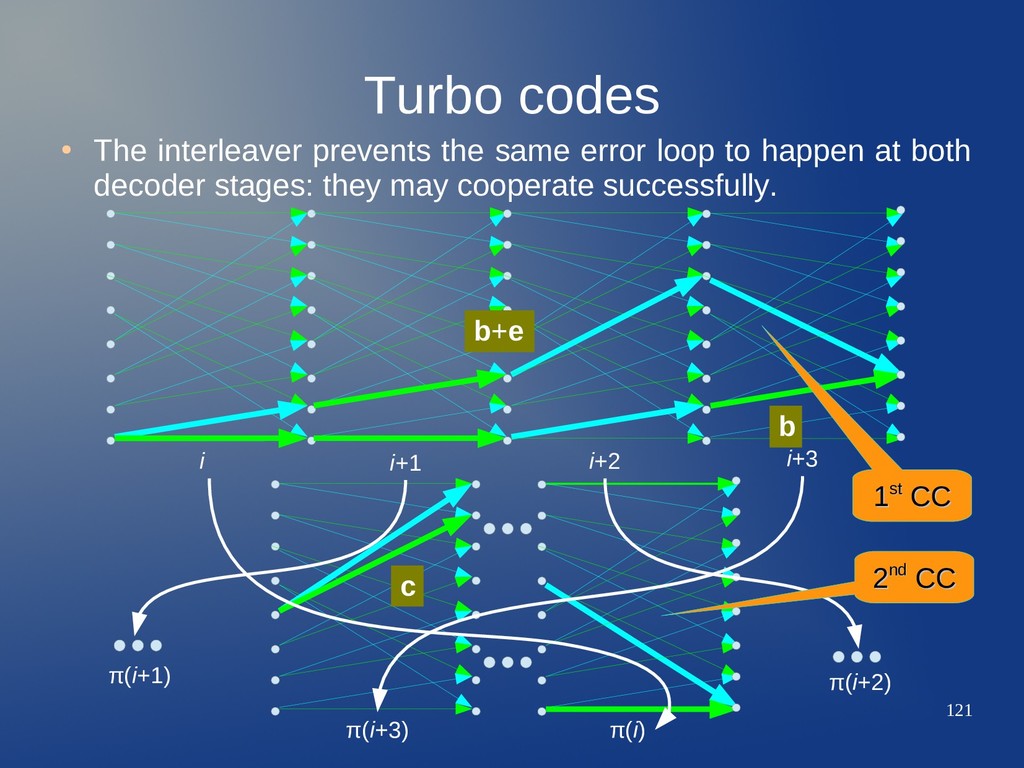
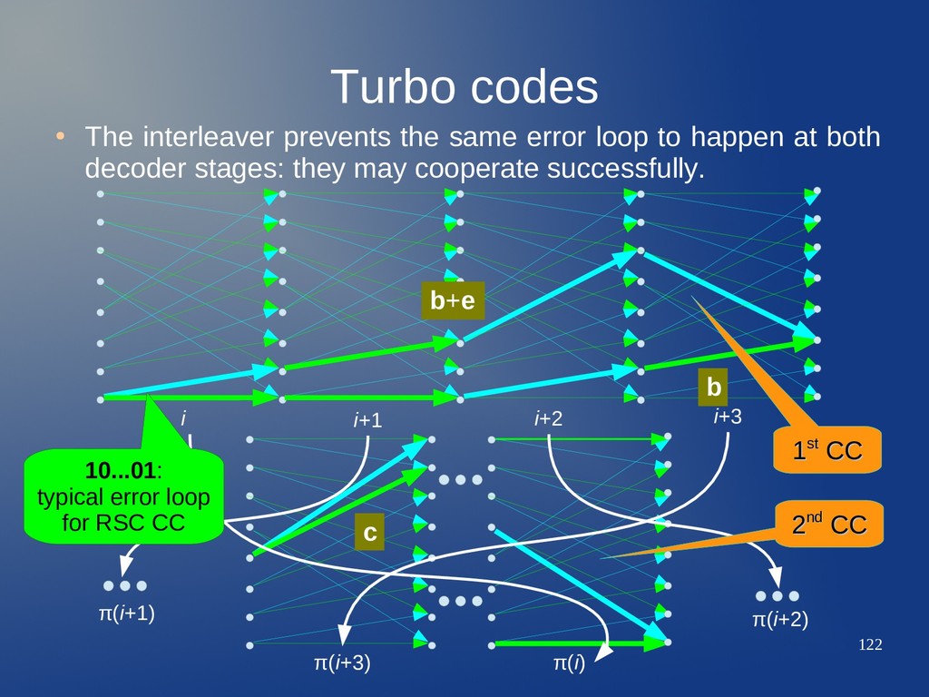
loop to happen at both decoder stages: they may cooperate successfully. b b+e i i+1 i+2 i+3 π(i+3) π(i) 1 1st st CC CC 10...01: typical error loop for RSC CC 2 2nd nd CC CC c π(i+2) π(i+1)
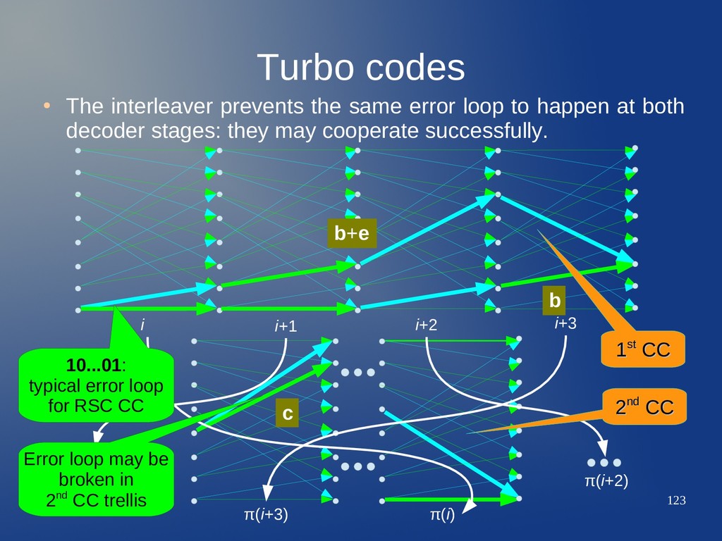
loop to happen at both decoder stages: they may cooperate successfully. b b+e i i+1 i+2 i+3 π(i+3) π(i) 1 1st st CC CC 10...01: typical error loop for RSC CC 2 2nd nd CC CC c π(i+2) π(i+1) Error loop may be broken in 2nd CC trellis
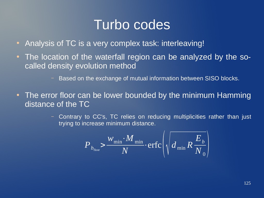
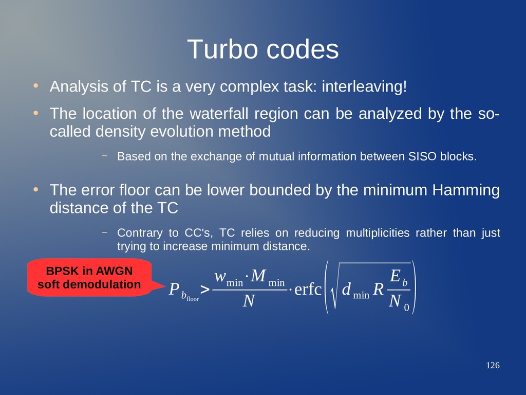
complex task: interleaving! • The location of the waterfall region can be analyzed by the so- called density evolution method – Based on the exchange of mutual information between SISO blocks. • The error floor can be lower bounded by the minimum Hamming distance of the TC – Contrary to CC's, TC relies on reducing multiplicities rather than just trying to increase minimum distance. P b floor > w min ⋅M min N ⋅erfc (√d min R E b N 0 )
complex task: interleaving! • The location of the waterfall region can be analyzed by the so- called density evolution method – Based on the exchange of mutual information between SISO blocks. • The error floor can be lower bounded by the minimum Hamming distance of the TC – Contrary to CC's, TC relies on reducing multiplicities rather than just trying to increase minimum distance. P b floor > w min ⋅M min N ⋅erfc (√d min R E b N 0 ) BPSK in AWGN soft demodulation
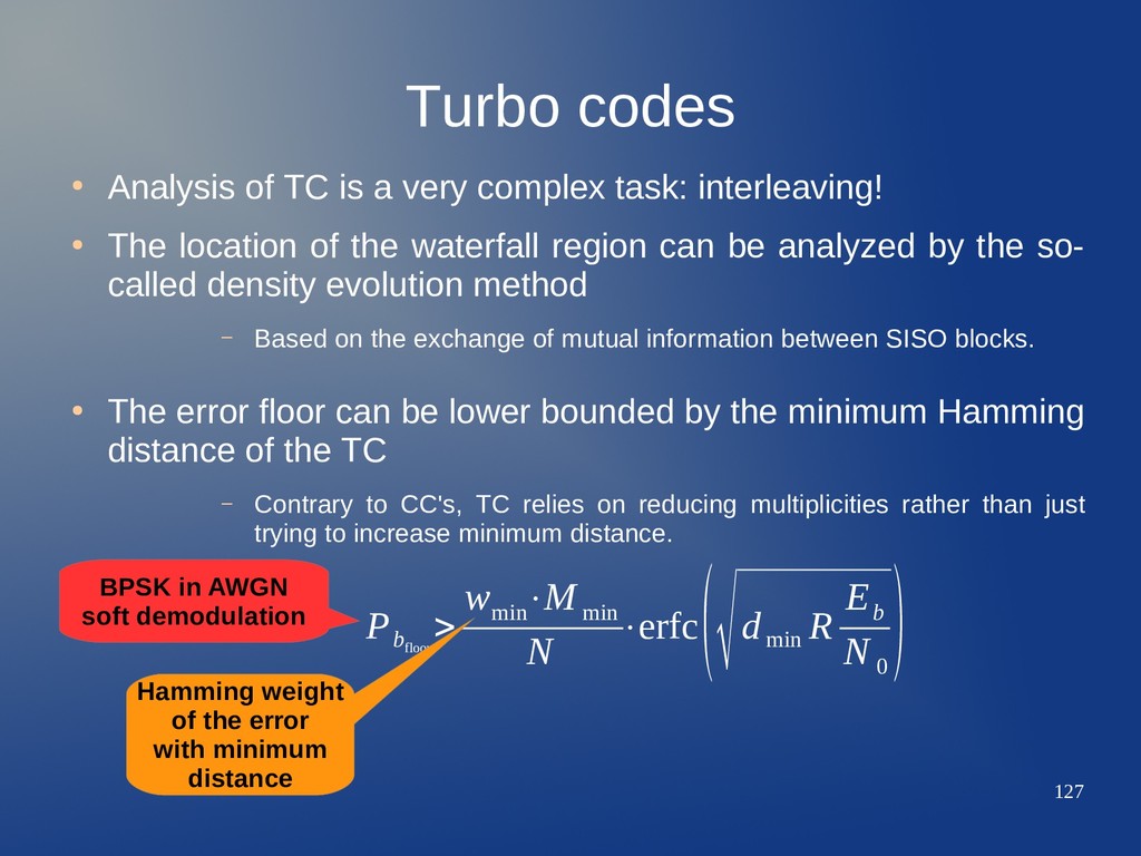
complex task: interleaving! • The location of the waterfall region can be analyzed by the so- called density evolution method – Based on the exchange of mutual information between SISO blocks. • The error floor can be lower bounded by the minimum Hamming distance of the TC – Contrary to CC's, TC relies on reducing multiplicities rather than just trying to increase minimum distance. P b floor > w min ⋅M min N ⋅erfc (√d min R E b N 0 ) Hamming weight of the error with minimum distance BPSK in AWGN soft demodulation
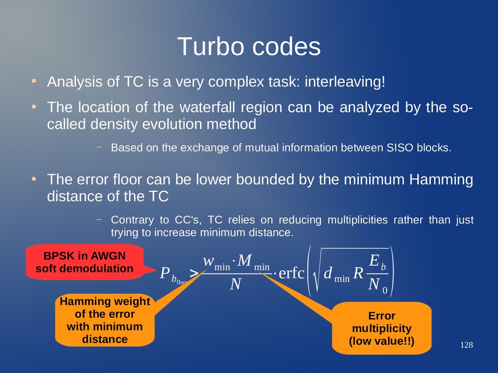
complex task: interleaving! • The location of the waterfall region can be analyzed by the so- called density evolution method – Based on the exchange of mutual information between SISO blocks. • The error floor can be lower bounded by the minimum Hamming distance of the TC – Contrary to CC's, TC relies on reducing multiplicities rather than just trying to increase minimum distance. P b floor > w min ⋅M min N ⋅erfc (√d min R E b N 0 ) Hamming weight of the error with minimum distance Error multiplicity (low value!!) BPSK in AWGN soft demodulation
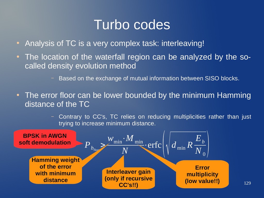
complex task: interleaving! • The location of the waterfall region can be analyzed by the so- called density evolution method – Based on the exchange of mutual information between SISO blocks. • The error floor can be lower bounded by the minimum Hamming distance of the TC – Contrary to CC's, TC relies on reducing multiplicities rather than just trying to increase minimum distance. P b floor > w min ⋅M min N ⋅erfc (√d min R E b N 0 ) Hamming weight of the error with minimum distance Error multiplicity (low value!!) Interleaver gain (only if recursive CC's!!) BPSK in AWGN soft demodulation
just another kind of channel codes derived from less complex ones. – While TC's were initially an extension of CC systems, LDPC codes are an extension of the concept of binary LBC, but they are not exactly our known LBC. • Formally, an LDPC code is an LBC whose parity check matrix is large and sparse. – Almost all matrix elements are 0!!!!!!!!!! – Very often, the LDPC parity check matrices are randomly generated, subject to some constraints on sparsity... – Recall that LBC relied on extreme powerful algebra related to carefully and well chosen matrix structures.
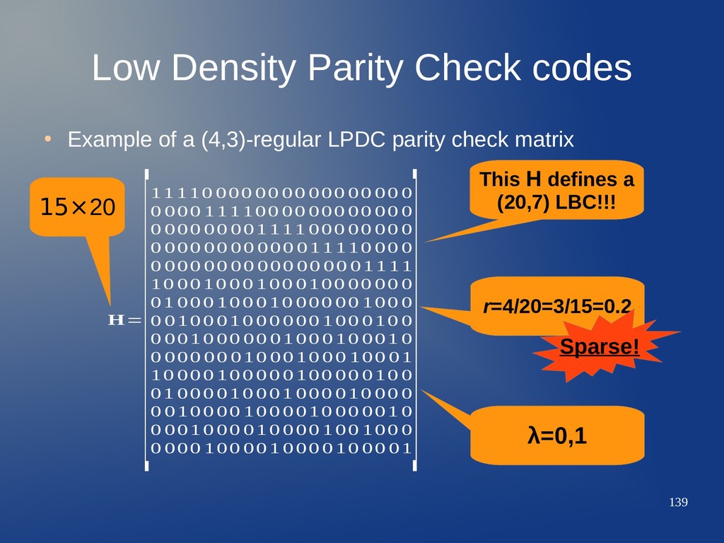
LDPC code is defined as the null space of a parity check matrix J⨯n H that meets these constraints: a) Each row contains ρ 1's. b) Each column contains γ 1's. c) λ, the number of 1's in common between any two columns, is 0 or 1. d) ρ and γ are small compared with n and J. • These properties give name to this class of codes: their matrices have a low density of 1's. • The density r of H is defined as r=ρ/n=γ/J.
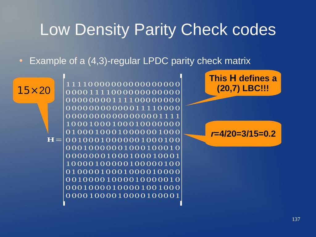
J rows of H are not necessarily linearly independent over GF(2). – To determine the dimension k of the code, it is mandatory to find the row rank of H = n-k < J. – That's the reason why in the previous example H defined a (20,7) LBC instead of a (20,5) LBC as could be expected! • The construction of large H for LDPC with high rates and good properties is a complex subject. – Some methods relay on smaller H i used as building blocks, plus random permutations or combinatorial manipulations; resulting matrices with bad properties are discarded. – Other methods relay on finite geometries and lot of algebra.
performances equal or even better than TC's, but without the problem of their relatively high error floor. – Both LDPC codes and TC's are capacity approaching codes. • As in the case of TC, their interest is in part related to the fact that – The encoding may be easily done, under some constraints (even if H is large, the low density of 1's may help reducing the complexity of the encoder). – At the decoder side, there are powerful algorithms that can take full advantage of the properties of the LDPC code.
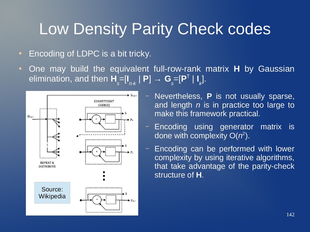
is a bit tricky. • One may build the equivalent full-row-rank matrix H by Gaussian elimination, and then H s =[I n-k | P] → G s =[PT | I k ]. – Nevertheless, P is not usually sparse, and length n is in practice too large to make this framework practical. – Encoding using generator matrix is done with complexity O(n2). – Encoding can be performed with lower complexity by using iterative algorithms, that take advantage of the parity-check structure of H. – Using G s Source: Wikipedia
is a bit tricky. • One may build the equivalent full-row-rank matrix H by Gaussian elimination, and then H s =[I n-k | P] → G s =[PT | I k ]. – Nevertheless, P is not usually sparse, and length n is in practice too large to make this framework practical. – Encoding using generator matrix is done with complexity O(n2). – Encoding can be performed with lower complexity by using iterative algorithms, that take advantage of the parity-check structure of H. – Using G s E.g. info bits are distributed through an structure with a lattice of simple encoders reproducing “local” parity-check equations Source: Wikipedia
algorithms to decode LDPC codes. – Hard decoding. – Soft decoding. – Mixed approaches. • We are going to examine two important instances thereof: – Majority-logic (MLG) decoding; hard decoding, the simplest one (lowest complexity). – Sum-product algorithm (SPA); soft decoding, best error performance (but high complexity!). • Key concepts: Tanner graphs & belief propagation.
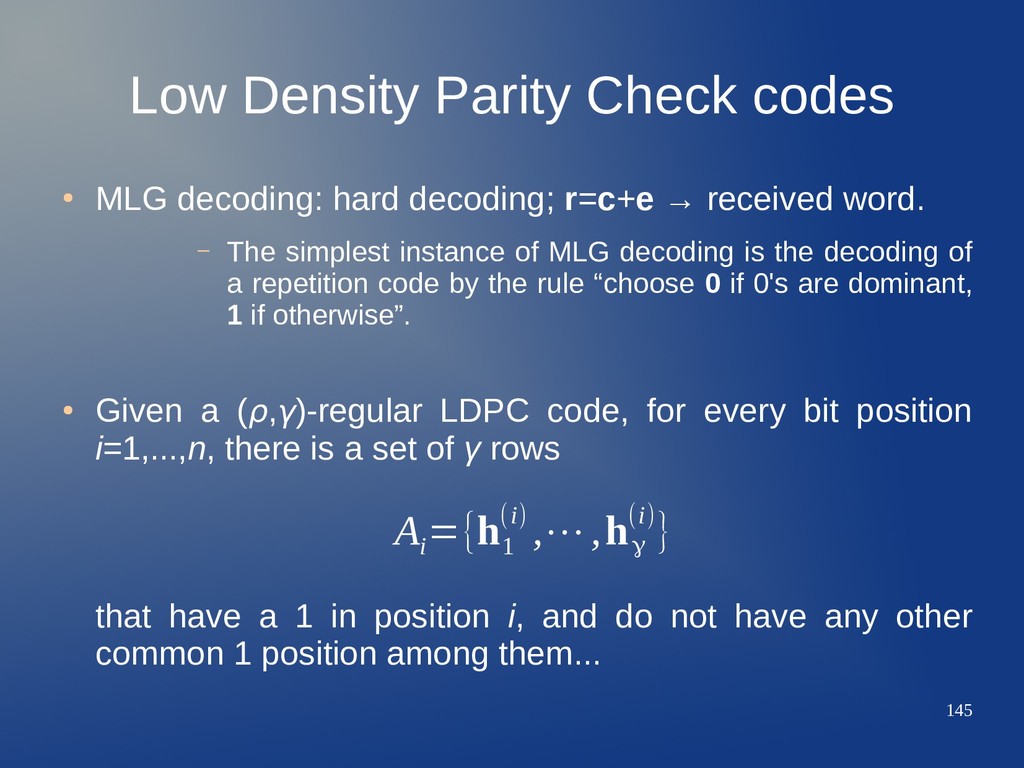
decoding; r=c+e → received word. – The simplest instance of MLG decoding is the decoding of a repetition code by the rule “choose 0 if 0's are dominant, 1 if otherwise”. • Given a (ρ,γ)-regular LDPC code, for every bit position i=1,...,n, there is a set of γ rows that have a 1 in position i, and do not have any other common 1 position among them... A i ={h 1 (i) ,⋯,h γ (i)}
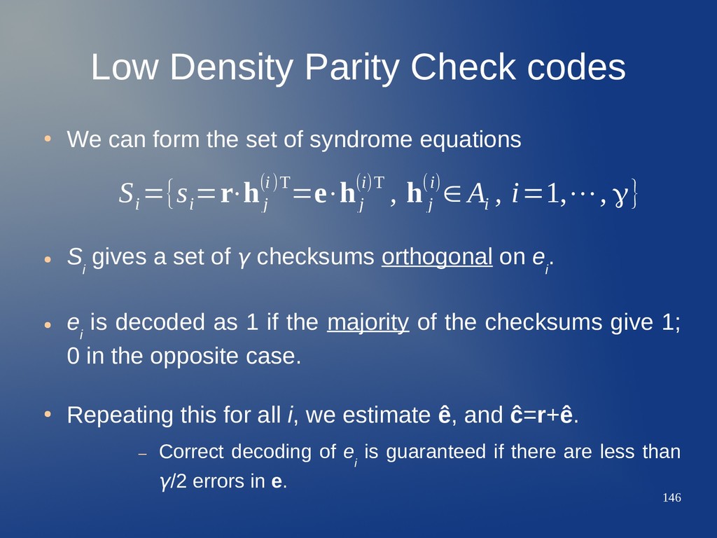
the set of syndrome equations • S i gives a set of γ checksums orthogonal on e i . • e i is decoded as 1 if the majority of the checksums give 1; 0 in the opposite case. • Repeating this for all i, we estimate ê, and ĉ=r+ê. – Correct decoding of e i is guaranteed if there are less than γ/2 errors in e. S i ={s i =r⋅h j (i)T =e⋅h j (i)T , h j (i)∈ A i , i=1,⋯, γ}
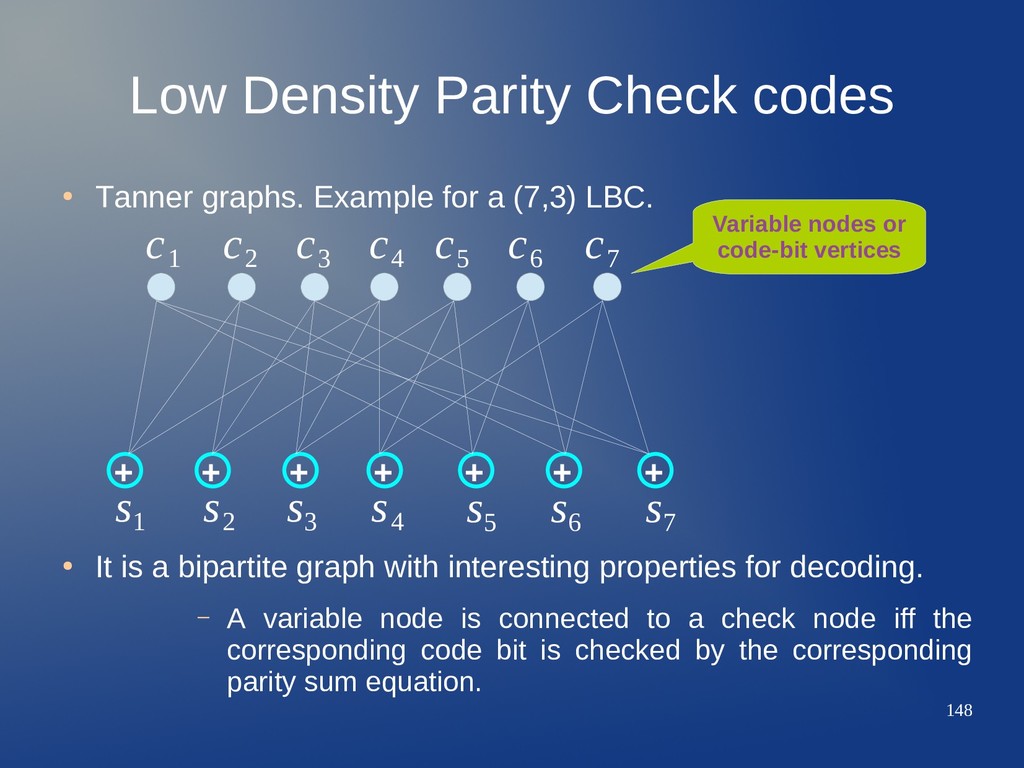
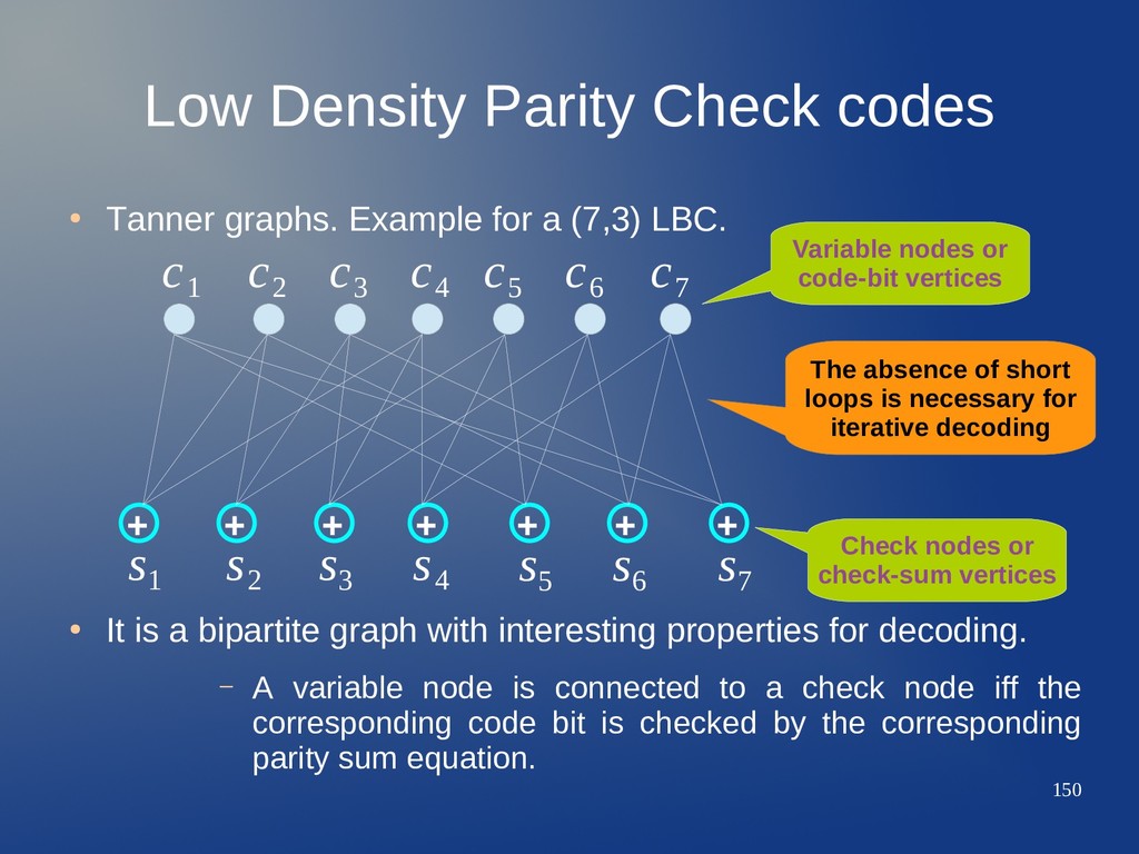
for a (7,3) LBC. • It is a bipartite graph with interesting properties for decoding. – A variable node is connected to a check node iff the corresponding code bit is checked by the corresponding parity sum equation. + + + + + + + c 1 c 2 c 3 c 4 c 5 c 6 c 7 s 1 s 2 s 3 s 4 s 5 s 6 s 7
for a (7,3) LBC. • It is a bipartite graph with interesting properties for decoding. – A variable node is connected to a check node iff the corresponding code bit is checked by the corresponding parity sum equation. + + + + + + + c 1 c 2 c 3 c 4 c 5 c 6 c 7 s 1 s 2 s 3 s 4 s 5 s 6 s 7 Variable nodes or code-bit vertices
for a (7,3) LBC. • It is a bipartite graph with interesting properties for decoding. – A variable node is connected to a check node iff the corresponding code bit is checked by the corresponding parity sum equation. + + + + + + + c 1 c 2 c 3 c 4 c 5 c 6 c 7 s 1 s 2 s 3 s 4 s 5 s 6 s 7 Variable nodes or code-bit vertices Check nodes or check-sum vertices
for a (7,3) LBC. • It is a bipartite graph with interesting properties for decoding. – A variable node is connected to a check node iff the corresponding code bit is checked by the corresponding parity sum equation. + + + + + + + c 1 c 2 c 3 c 4 c 5 c 6 c 7 s 1 s 2 s 3 s 4 s 5 s 6 s 7 Variable nodes or code-bit vertices Check nodes or check-sum vertices The absence of short loops is necessary for iterative decoding
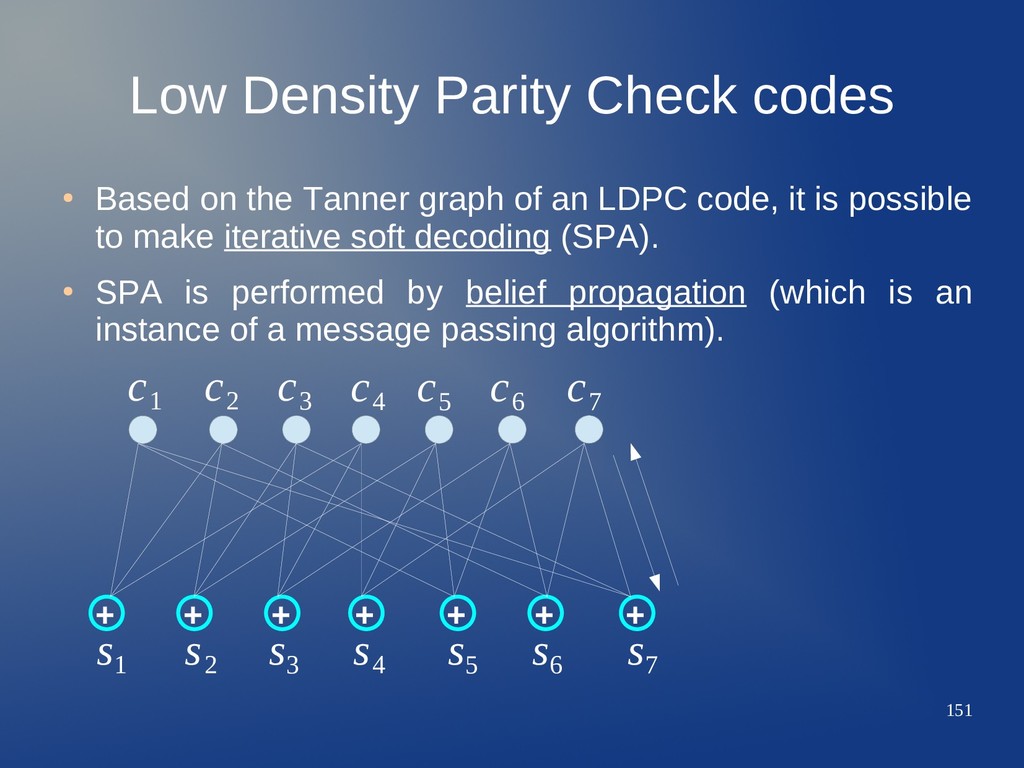
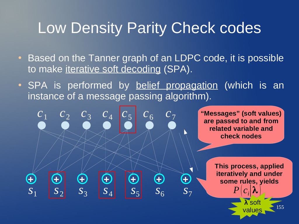
Tanner graph of an LDPC code, it is possible to make iterative soft decoding (SPA). • SPA is performed by belief propagation (which is an instance of a message passing algorithm). + + + + + + + c 1 c 2 c 3 c 4 c 5 c 6 c 7 s 1 s 2 s 3 s 4 s 5 s 6 s 7
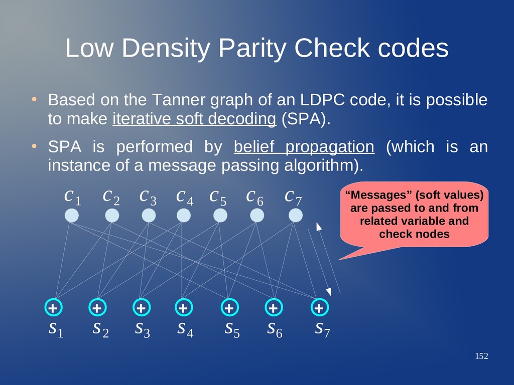
Tanner graph of an LDPC code, it is possible to make iterative soft decoding (SPA). • SPA is performed by belief propagation (which is an instance of a message passing algorithm). + + + + + + + c 1 c 2 c 3 c 4 c 5 c 6 c 7 s 1 s 2 s 3 s 4 s 5 s 6 s 7 “Messages” (soft values) are passed to and from related variable and check nodes
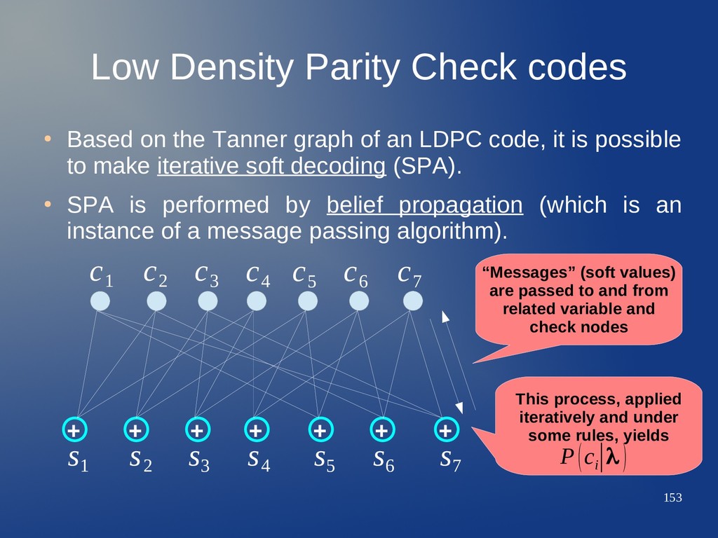
Tanner graph of an LDPC code, it is possible to make iterative soft decoding (SPA). • SPA is performed by belief propagation (which is an instance of a message passing algorithm). + + + + + + + c 1 c 2 c 3 c 4 c 5 c 6 c 7 s 1 s 2 s 3 s 4 s 5 s 6 s 7 “Messages” (soft values) are passed to and from related variable and check nodes This process, applied iteratively and under some rules, yields P(c i ∣λ )
Tanner graph of an LDPC code, it is possible to make iterative soft decoding (SPA). • SPA is performed by belief propagation (which is an instance of a message passing algorithm). + + + + + + + c 1 c 2 c 3 c 4 c 5 c 6 c 7 s 1 s 2 s 3 s 4 s 5 s 6 s 7 “Messages” (soft values) are passed to and from related variable and check nodes This process, applied iteratively and under some rules, yields P(c i ∣λ ) λ soft values
Tanner graph of an LDPC code, it is possible to make iterative soft decoding (SPA). • SPA is performed by belief propagation (which is an instance of a message passing algorithm). + + + + + + + c 1 c 2 c 3 c 4 c 5 c 6 c 7 s 1 s 2 s 3 s 4 s 5 s 6 s 7 “Messages” (soft values) are passed to and from related variable and check nodes This process, applied iteratively and under some rules, yields P(c i ∣λ ) λ soft values
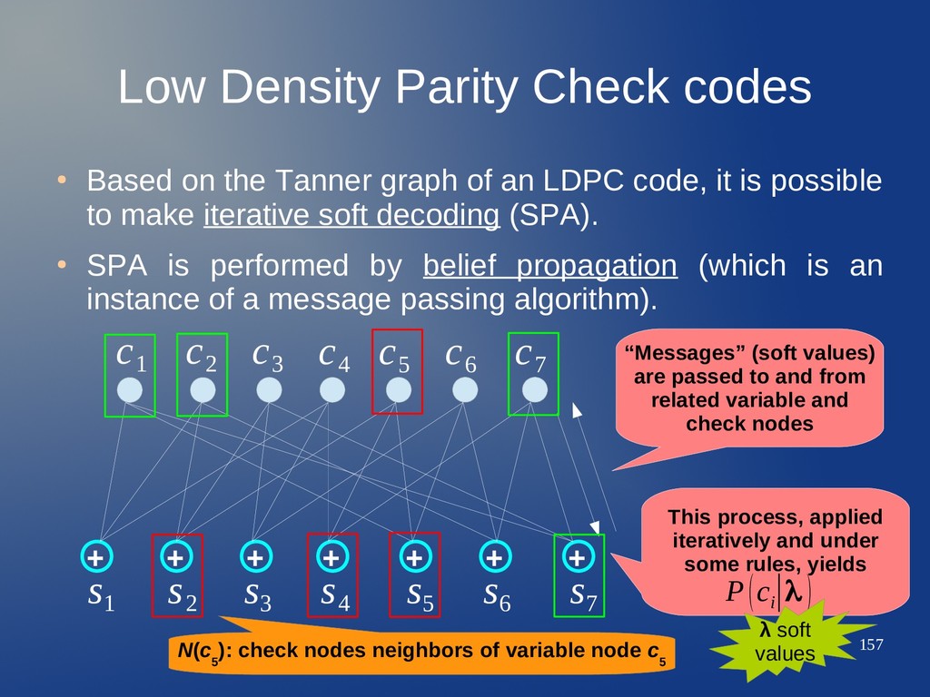
Tanner graph of an LDPC code, it is possible to make iterative soft decoding (SPA). • SPA is performed by belief propagation (which is an instance of a message passing algorithm). + + + + + + + c 1 c 2 c 3 c 4 c 5 c 6 c 7 s 1 s 2 s 3 s 4 s 5 s 6 s 7 “Messages” (soft values) are passed to and from related variable and check nodes This process, applied iteratively and under some rules, yields P(c i ∣λ ) N(c 5 ): check nodes neighbors of variable node c 5 λ soft values
Tanner graph of an LDPC code, it is possible to make iterative soft decoding (SPA). • SPA is performed by belief propagation (which is an instance of a message passing algorithm). + + + + + + + c 1 c 2 c 3 c 4 c 5 c 6 c 7 s 1 s 2 s 3 s 4 s 5 s 6 s 7 “Messages” (soft values) are passed to and from related variable and check nodes This process, applied iteratively and under some rules, yields P(c i ∣λ ) N(c 5 ): check nodes neighbors of variable node c 5 λ soft values
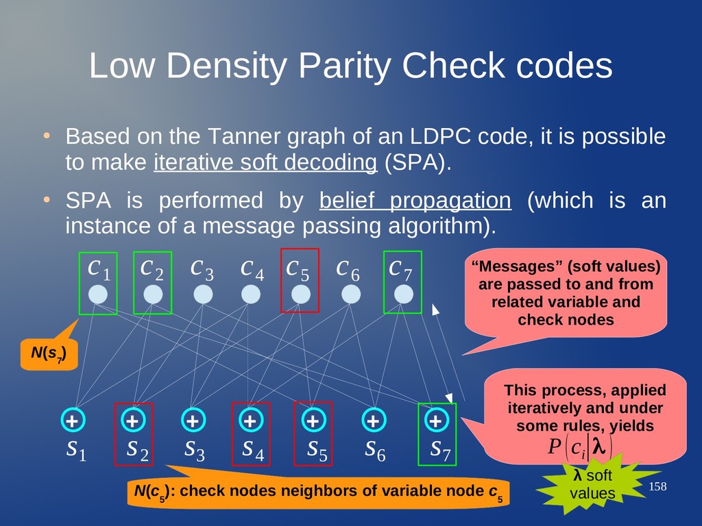
Tanner graph of an LDPC code, it is possible to make iterative soft decoding (SPA). • SPA is performed by belief propagation (which is an instance of a message passing algorithm). + + + + + + + c 1 c 2 c 3 c 4 c 5 c 6 c 7 s 1 s 2 s 3 s 4 s 5 s 6 s 7 “Messages” (soft values) are passed to and from related variable and check nodes This process, applied iteratively and under some rules, yields P(c i ∣λ ) N(c 5 ): check nodes neighbors of variable node c 5 N(s 7 ) λ soft values
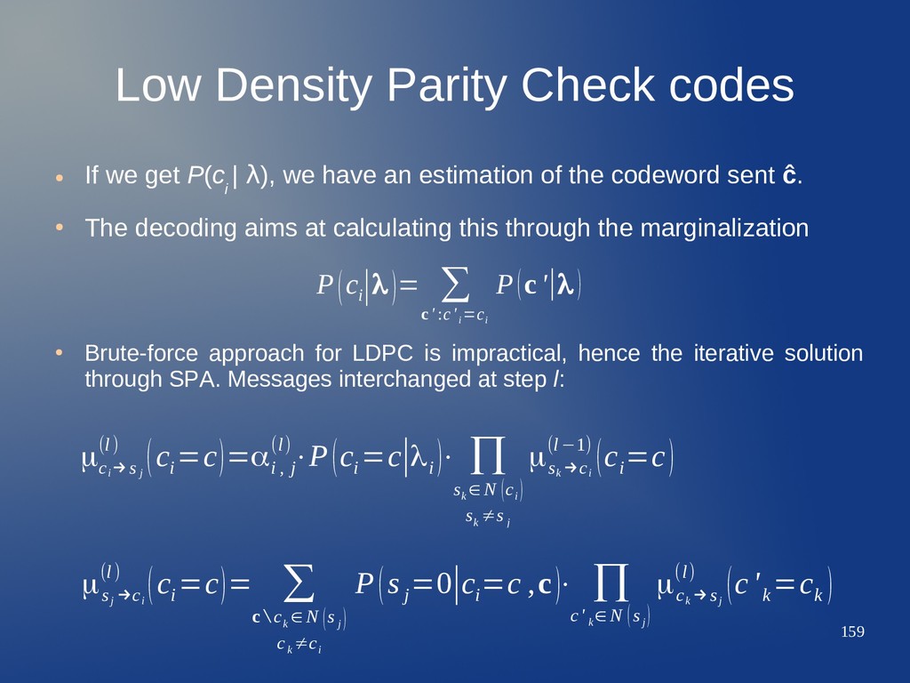
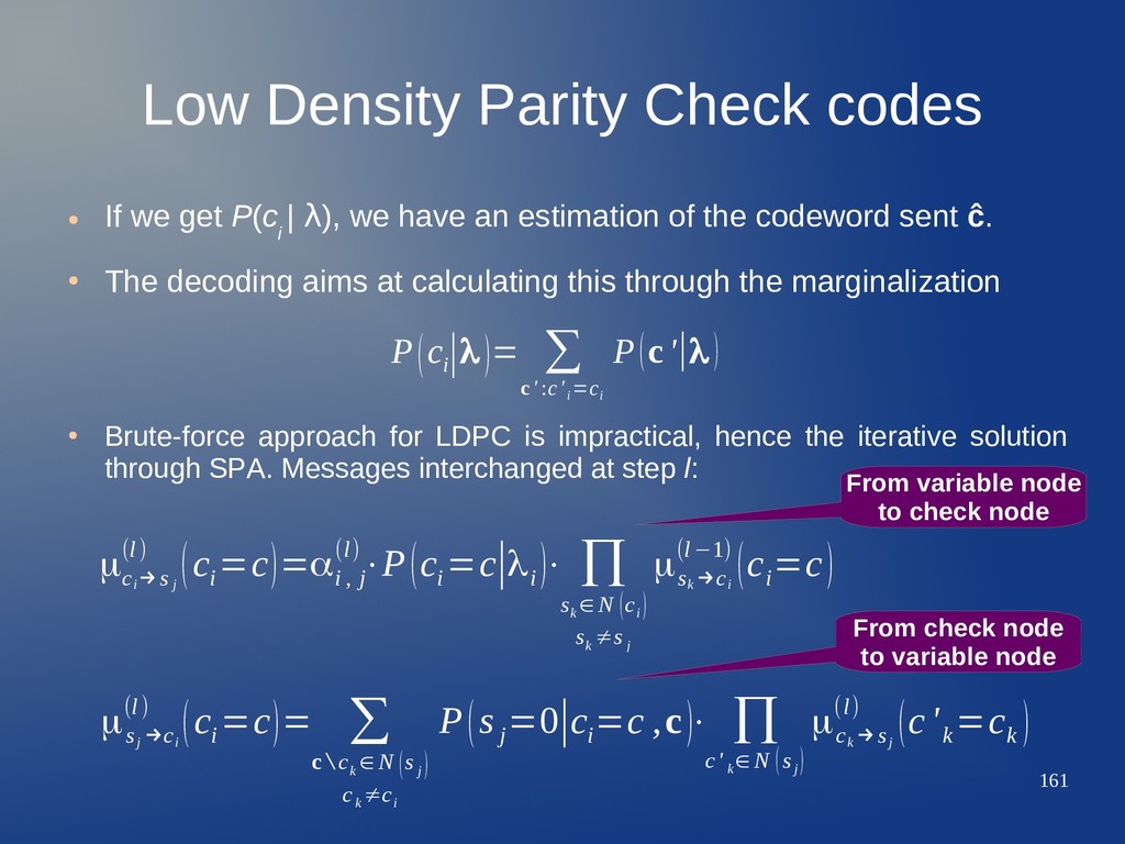
P(c i | λ), we have an estimation of the codeword sent ĉ. • The decoding aims at calculating this through the marginalization • Brute-force approach for LDPC is impractical, hence the iterative solution through SPA. Messages interchanged at step l: P(c i ∣λ)= ∑ c' :c' i =c i P(c '∣λ) μc i →s j (l) (c i =c)=αi , j (l)⋅P(c i =c∣λi )⋅ ∏ s k ∈N (c i ) s k ≠s j μs k →c i (l−1) (c i =c) μs j →c i (l) (c i =c)= ∑ c∖c k ∈N (s j ) c k ≠c i P(s j =0∣c i =c ,c)⋅ ∏ c' k ∈N (s j ) μc k →s j (l) (c ' k =c k )
P(c i | λ), we have an estimation of the codeword sent ĉ. • The decoding aims at calculating this through the marginalization • Brute-force approach for LDPC is impractical, hence the iterative solution through SPA. Messages interchanged at step l: P(c i ∣λ)= ∑ c' :c' i =c i P(c '∣λ) μc i →s j (l) (c i =c)=αi , j (l)⋅P(c i =c∣λi )⋅ ∏ s k ∈N (c i ) s k ≠s j μs k →c i (l−1) (c i =c) μs j →c i (l) (c i =c)= ∑ c∖c k ∈N (s j ) c k ≠c i P(s j =0∣c i =c ,c)⋅ ∏ c' k ∈N (s j ) μc k →s j (l) (c ' k =c k ) From variable node to check node
P(c i | λ), we have an estimation of the codeword sent ĉ. • The decoding aims at calculating this through the marginalization • Brute-force approach for LDPC is impractical, hence the iterative solution through SPA. Messages interchanged at step l: P(c i ∣λ)= ∑ c' :c' i =c i P(c '∣λ) μc i →s j (l) (c i =c)=αi , j (l)⋅P(c i =c∣λi )⋅ ∏ s k ∈N (c i ) s k ≠s j μs k →c i (l−1) (c i =c) μs j →c i (l) (c i =c)= ∑ c∖c k ∈N (s j ) c k ≠c i P(s j =0∣c i =c ,c)⋅ ∏ c' k ∈N (s j ) μc k →s j (l) (c ' k =c k ) From variable node to check node From check node to variable node
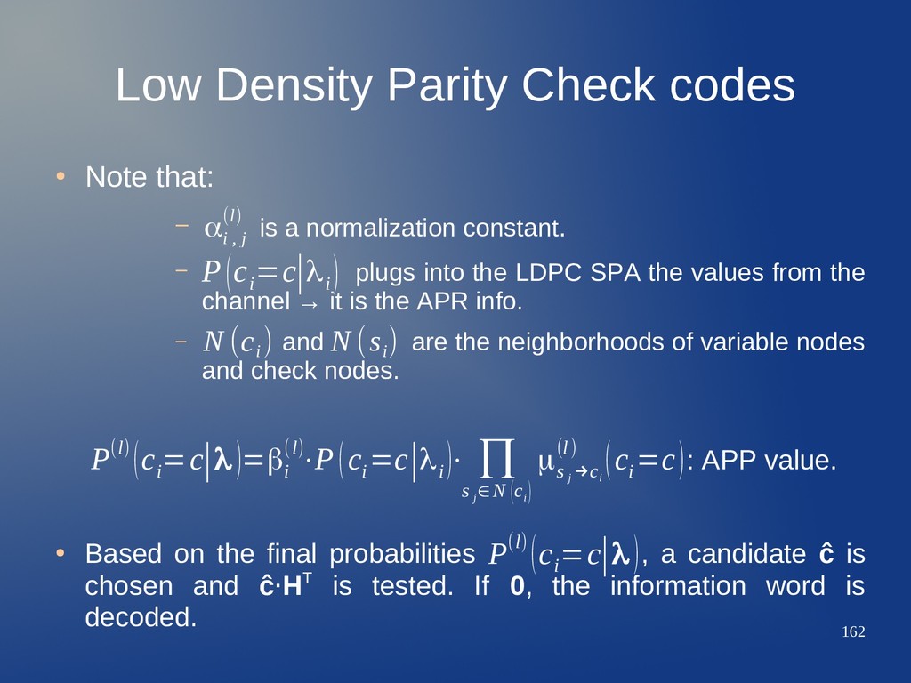
is a normalization constant. – plugs into the LDPC SPA the values from the channel → it is the APR info. – and are the neighborhoods of variable nodes and check nodes. : APP value. • Based on the final probabilities , a candidate ĉ is chosen and ĉ·HT is tested. If 0, the information word is decoded. αi , j (l) P(c i =c|λi ) P(l) (c i =c|λ)=βi (l) ⋅P(c i =c|λi )⋅ ∏ s j ∈N (c i ) μs j →c i (l) (c i =c) N (c i ) N (s i ) P(l) (c i =c|λ)
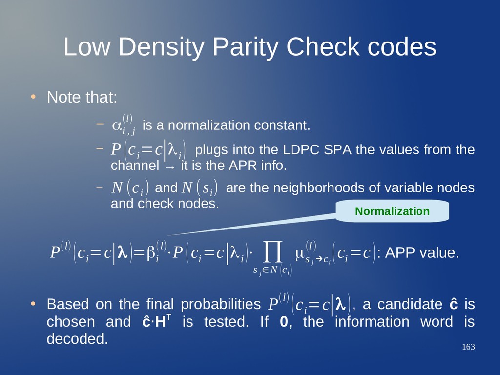
is a normalization constant. – plugs into the LDPC SPA the values from the channel → it is the APR info. – and are the neighborhoods of variable nodes and check nodes. : APP value. • Based on the final probabilities , a candidate ĉ is chosen and ĉ·HT is tested. If 0, the information word is decoded. αi , j (l) P(c i =c|λi ) P(l) (c i =c|λ)=βi (l) ⋅P(c i =c|λi )⋅ ∏ s j ∈N (c i ) μs j →c i (l) (c i =c) Normalization N (c i ) N (s i ) P(l) (c i =c|λ)
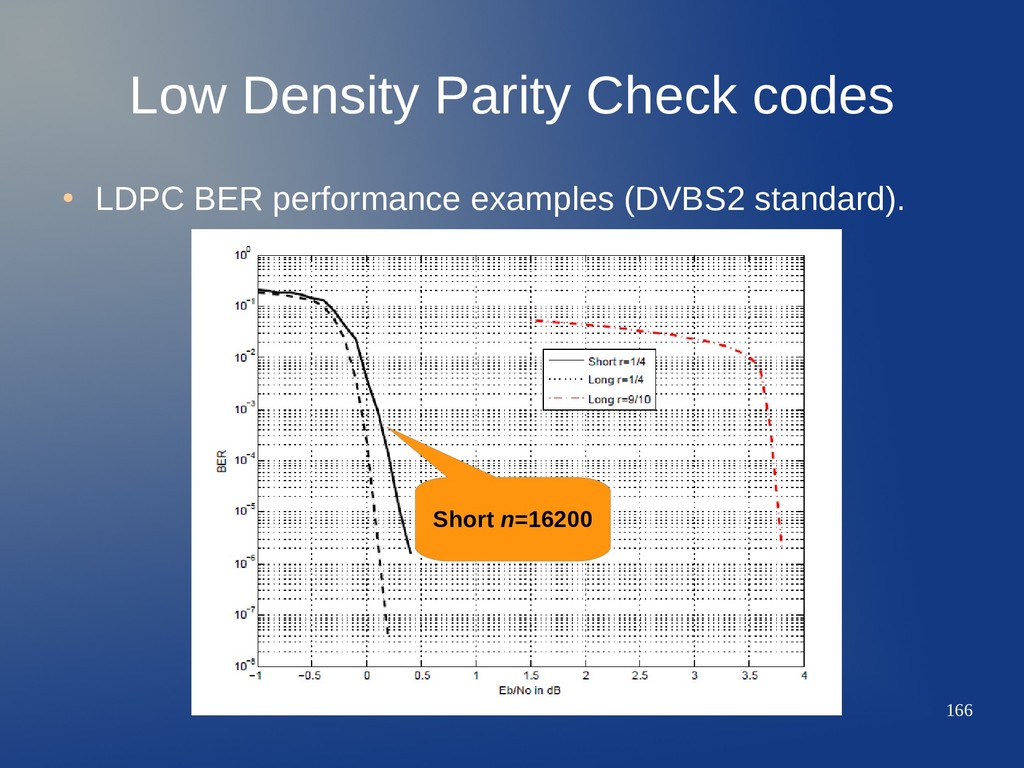
the possibility to analyze their performance. – They have also error floors that may be characterized, on the basis of their minimum distance. – Good performance is related with sparsity (it breaks error recurrences along parity check equations). • Analysis techniques are complex. – They require taking into account the Tanner graph structure, nature of their loops, and so on. – It is possible to draw bounds for the BER, and give design and evaluation criteria thereon. – Analysis depends heavily on the nature of the LDPC: regular, irregular..., and constitutes a field of very active research.
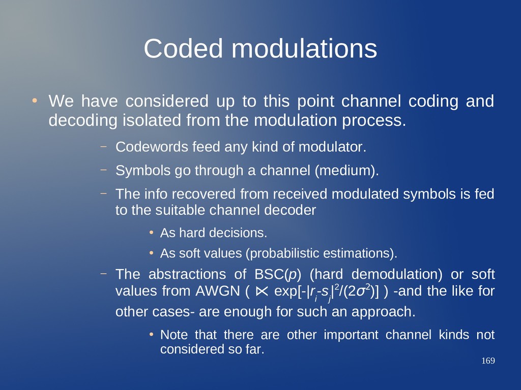
point channel coding and decoding isolated from the modulation process. – Codewords feed any kind of modulator. – Symbols go through a channel (medium). – The info recovered from received modulated symbols is fed to the suitable channel decoder • As hard decisions. • As soft values (probabilistic estimations). – The abstractions of BSC(p) (hard demodulation) or soft values from AWGN ( ⋉ there iexp[-|r i -s j |2/(2σ2)] ) -and the like for other cases- are enough for such an approach. • Note that there are other important channel kinds not considered so far.
coding and modulation are treated as a whole. – Joint coding/modulation. – Joint decoding/demodulation. • This offers potential advantages (recall the improvements made when the demodulator outputs more elaborated information -soft values vs. hard decisions). – We combine gains in BER with spectral efficiency! • As a drawback, the systems become more complex. – More difficult to design and analyze.
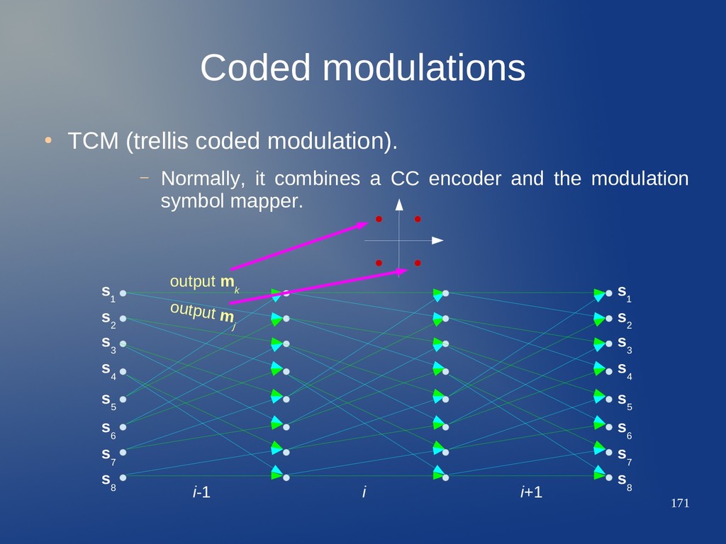
it combines a CC encoder and the modulation symbol mapper. output m k output m j s 2 s 1 s 3 s 4 s 6 s 5 s 7 s 8 s 2 s 3 s 4 s 6 s 5 s 7 s 8 s 1 i-1 i i+1
well matched to the CC trellis, and the decoder is accordingly designed to take advantage of it, – TCM provides high spectral efficiency. – TCM can be robust in AWGN channels, and against fading and multipath effects. • In the 80's, TCM become the standard for telephone line data modems. – No other system could provide better performance over the twisted pair cable before the introduction of DMT and ADSL. • However, the flexibility of providing separated channel coding and modulation subsystems is still preferred nowadays. – Under the concept of Adaptive Coding & Modulation (ACM).
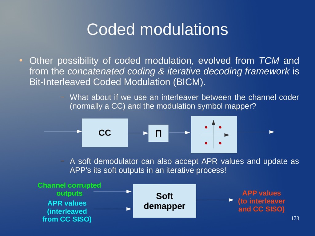
from TCM and from the concatenated coding & iterative decoding framework is Bit-Interleaved Coded Modulation (BICM). – What about if we use an interleaver between the channel coder (normally a CC) and the modulation symbol mapper? – A soft demodulator can also accept APR values and update as APP's its soft outputs in an iterative process! CC Π Soft demapper Channel corrupted outputs APR values (interleaved from CC SISO) APP values (to interleaver and CC SISO)
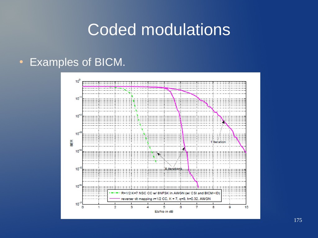
behavior (even better!) – In channels where spectral efficiency is required. – In dispersive channels (multipath, fading). – Iterative decoding yields a steep waterfall region. – Being a serial concatenated system, the error floor is very low (contrary to the parallel concatenated systems). • BICM has already found applications in standards such as DVB-T2. • The drawback is the higher latency and complexity of the decoding.
for modern digital communications. – All standards at the PHY level include one or more channel coding methods. – Modulation & coding are usually considered together to guarantee a final performance level. • Error control comes out in two main flavors: ARQ and FEC. – Nevertheless, hybrid strategies are becoming more and more popular (HARQ). • A lot of research has been made, with successful results, to approach Shannon's promises from the noisy-channel coding theorem. • Concatenation and iterative (soft) decoding are pushing the results towards channel capacity.
of codes endowed with less rich algebraic structure, and relaying more on statistical / probabilistic grounds. • New outstanding proposals are being made, relaying more intensively on randomness, as hinted by Shannon's demonstrations. – New capacity-achieving alternatives, like polar codes and fountain codes, are step-by-step reaching the market, with promising prospects. – Nonetheless, their processing needs make them more suitable for higher layers than the PHY. • Though we are already approaching the limits of the Gaussian channel, there are still many challenges. – In general, the wireless channel poses problems unresolved from the point of view of capacity calculation & exploitation through channel coding.
Prentice Hall, 2004. • S. B. Wicker, ERROR CONTROL SYSTEMS FOR DIGITAL COMMUNICATION AND STORAGE, Prentice Hall, 1995. • J. M. Cioffi, DIGITAL COMMUNICATIONS - CODING (course), Stanford University, 2010. [Online] Available: http://web.stanford.edu/group/cioffi/book