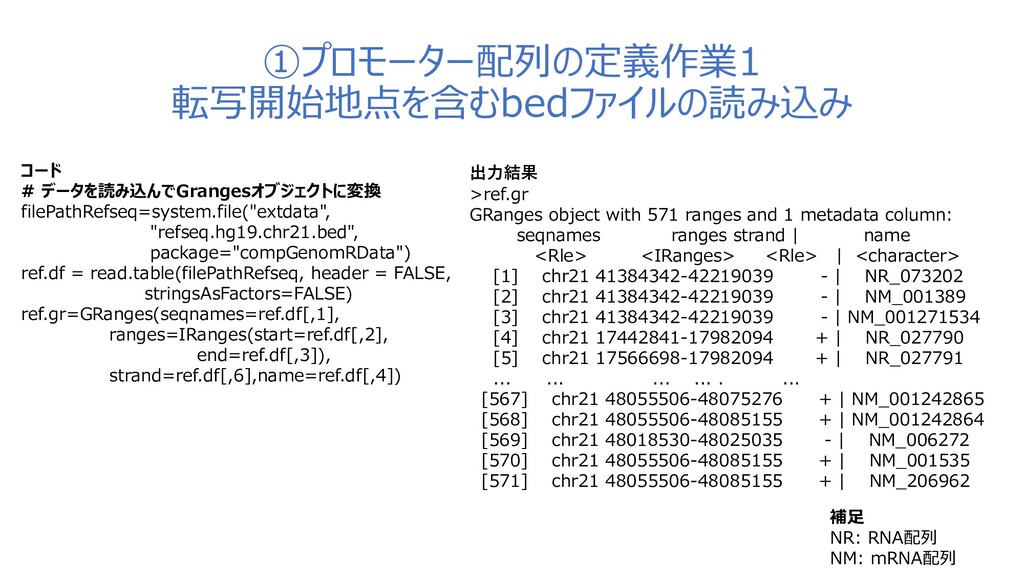
read.table(filePathRefseq, header = FALSE, stringsAsFactors=FALSE) ref.gr=GRanges(seqnames=ref.df[,1], ranges=IRanges(start=ref.df[,2], end=ref.df[,3]), strand=ref.df[,6],name=ref.df[,4]) 補足 NR: RNA配列 NM: mRNA配列 出力結果 >ref.gr GRanges object with 571 ranges and 1 metadata column: seqnames ranges strand | name <Rle> <IRanges> <Rle> | <character> [1] chr21 41384342-42219039 - | NR_073202 [2] chr21 41384342-42219039 - | NM_001389 [3] chr21 41384342-42219039 - | NM_001271534 [4] chr21 17442841-17982094 + | NR_027790 [5] chr21 17566698-17982094 + | NR_027791 ... ... ... ... . ... [567] chr21 48055506-48075276 + | NM_001242865 [568] chr21 48055506-48085155 + | NM_001242864 [569] chr21 48018530-48025035 - | NM_006272 [570] chr21 48055506-48085155 + | NM_001535 [571] chr21 48055506-48085155 + | NM_206962
![GRangesオブジェクトの使用に関して ①表データに近い扱いが可能 →gr[1:2,], gr$name1といった 特定のデータへのアクセスが可能 ➁基本のデータ以外にメタデータを追加可能 mcols(gr)=DataFrame(name1=c("pax6","meis1","zic4"), score2=c(1,2,3)) Rstudioの操作画面](https://files.speakerdeck.com/presentations/e71edbd834594ec1850588bca7d4ee38/slide_4.jpg)
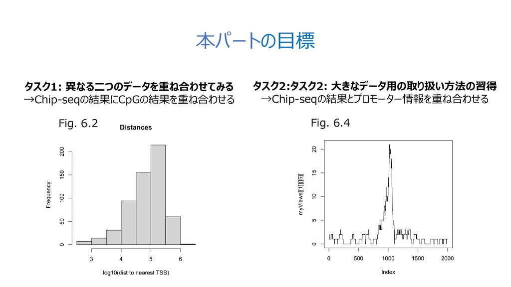
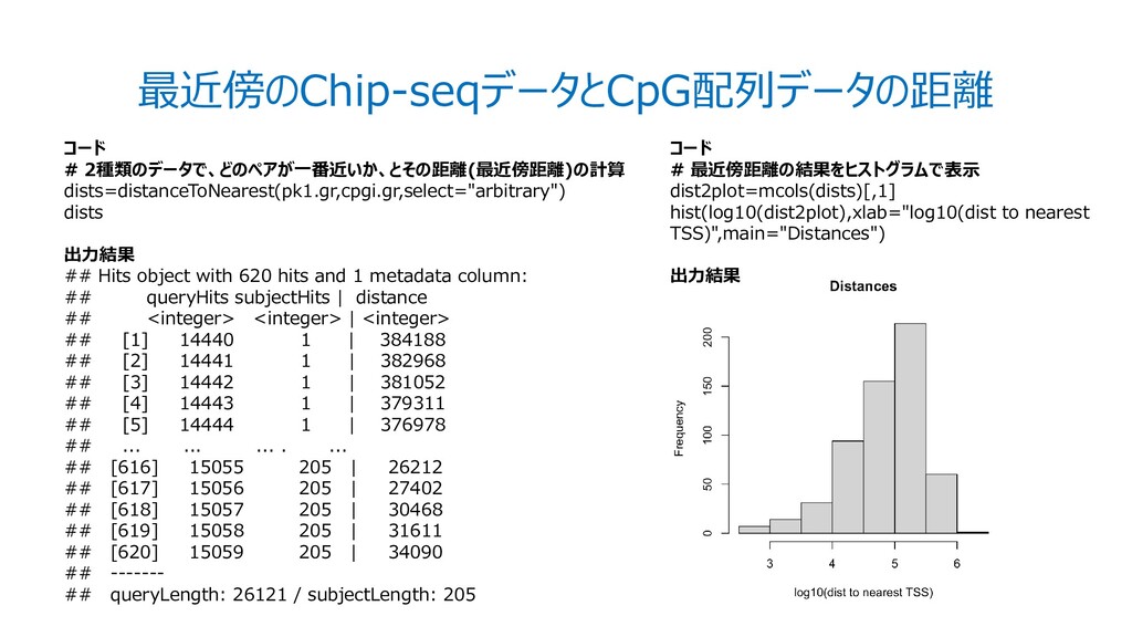
![テキスト中では距離をそのまま対数変換している #対数変換前のChip-seqとCpGデータの距離データ SP1_CpGDist=dists@elementMetadata@listData[["distance"]] > SP1_CpGDist [1] 384188 382968 381052 379311](https://files.speakerdeck.com/presentations/e71edbd834594ec1850588bca7d4ee38/slide_12.jpg)