On the estimation of the infection rate in epidemic models with multiple populations

Transcript

1. On the estimation of the infection rate in epidemic models with multiple populations Gianluca Campanella Imperial College London Isabel C. M. Nat´ ario Ricardo A. M. Pereira Universidade Nova de Lisboa Universit` a degli Studi di Trento VI International Workshop on Spatio-Temporal Modelling Guimar˜ aes, Portugal · September 12, 2012
2. Contents 1 Compartmental models 2 Estimation method 3 Results
3. Contents 1 Compartmental models 2 Estimation method 3 Results
4. Compartmental models SIR model of Kermack and McKendrick The SIR model of Kermack and McKendrick considers a closed population whose members are subdivided into three states: Susceptible Infectious Recovered S I R β γ β Infection rate γ Recovery rate (can be estimated clinically)
5. Compartmental models SIR model formulations in continuous time Deterministic (system of ODE) dS dt = −β S(t) I(t) dI dt = β S(t) I(t) − γ I(t) dR dt = γ I(t) Stochastic (Markov chain) (s, i) (s + 1, i − 1) (s, i + 1) β (s + 1) (i − 1) γ (i + 1)
6. Compartmental models Meta-population models • Each population is modelled by a compartmental model • Transportation network provides weak coupling Population i Si Ii Ri Population j Sj Ij Rj aij Ni aji Nj
7. Compartmental models Summary SIR model 1. Closed population 2. Three states (susceptible, infectious and recovered) 3. Two parameters (infection rate β and recovery rate γ) Meta-population models 1. Straightforward extension of compartmental models to multiple populations 2. Each population is modelled (almost) independently 3. Weak coupling provided by transportation network
8. Contents 1 Compartmental models 2 Estimation method 3 Results
9. Estimation method Main idea Hypotheses 1. initially, all infectious individuals belong to the same population 2. the disease reaches other populations by means of travels along the transportation network
10. Estimation method Main idea Hypotheses 1. initially, all infectious individuals belong to the same population 2. the disease reaches other populations by means of travels along the transportation network Main idea The time of arrival of the first infectious individual at each population depends on the parameters β and γ.
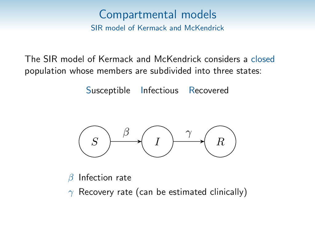
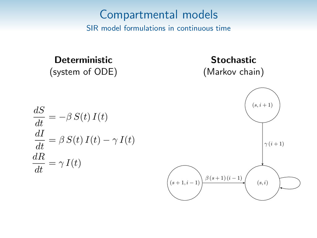
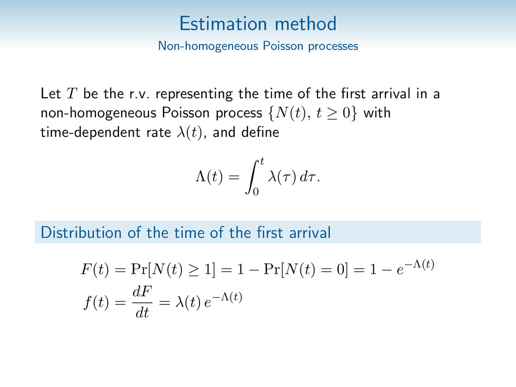
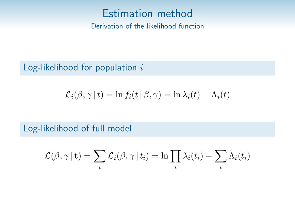
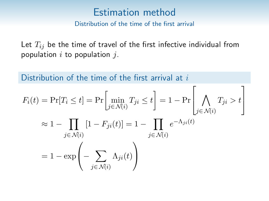
11. Estimation method Non-homogeneous Poisson processes Definition A counting process {N(t), t ≥ 0} is said to be a non-homogeneous Poisson process with time-dependent rate λ(t) ≥ 0, t ≥ 0, if the following conditions hold, 1. N(0) = 0, 2. {N(t), t ≥ 0} has independent increments, 3. Pr[N(t + h) − N(t) = 1] = λ(t) h + o(h), 4. Pr[N(t + h) − N(t) ≥ 2] = o(h), where o(h) is such that limh→ 0 o(h)/h = 0.
12. Estimation method Non-homogeneous Poisson processes Let T be the r.v. representing the time of the first arrival in a non-homogeneous Poisson process {N(t), t ≥ 0} with time-dependent rate λ(t), and define Λ(t) = t 0 λ(τ) dτ. Distribution of the time of the first arrival F(t) = Pr[N(t) ≥ 1] = 1 − Pr[N(t) = 0] = 1 − e−Λ(t) f(t) = dF dt = λ(t) e−Λ(t)
13. Estimation method Distribution of the time of the first arrival The arrival process of infectious individuals at population i is a non-homogeneous Poisson process, since: 1. initially, no infectious individuals are present; 2. travels (and thus increments) to i are independent; 3. the probability of arrival during h depends on the number of infectious individuals in neighbouring populations multiplied by the corresponding travel probabilities; 4. the probability of more than one arrival during h is negligible. Density of the time of the first arrival at i fi (t | β, γ) = λi (t) e−Λi(t), λi (t) = j∈ N(i) pji Ij (t | β, γ)
14. Estimation method Distribution of the time of the first arrival 0 50 100 150 200 0.000 0.005 0.010 0.015 0.020 0.025 0.030 0.08 0.1 0.12 0 50 100 150 200 0.000 0.005 0.010 0.015 0.020 0.025 0.030 0.04 0.05 0.06
15. Estimation method Derivation of the likelihood function Log-likelihood for population i Li (β, γ | t) = ln fi (t | β, γ) = ln λi (t) − Λi (t) Log-likelihood of full model L(β, γ | t) = i Li (β, γ | ti ) = ln i λi (ti ) − i Λi (ti )
16. Estimation method Summary Idea 1. Assume that disease is non-endemic 2. Times of arrival of first infectious individuals depend on model parameters β and γ Formalization 1. Arrivals at each population are non-homogeneous Poisson processes 2. The number of infectious individuals in neighbouring populations can be simulated, or approximated using the corresponding deterministic formulation
17. Contents 1 Compartmental models 2 Estimation method 3 Results
18. Results Simulation scenario: primary case in Ave • 28 continental Portugal subregions (NUTS 3 classification) • Resident and commuting population information provided by INE • Infection starts in Ave Norte Centro Lisboa Alentejo Algarve 0 50 100 150 200 250
19. Results Infection rate estimates for increasing number of recorded arrival times 2 3 4 5 6 7 8 9 0.0 0.1 0.2 0.3 0.4 0.5
20. Results Simulation scenario: primary case in Grande Lisboa • 28 continental Portugal subregions (NUTS 3 classification) • Resident and commuting population information provided by INE • Infection starts in Grande Lisboa Norte Centro Lisboa Alentejo Algarve 0 100 200 300
21. Results Infection rate estimates for increasing number of recorded arrival times 4 5 6 7 8 9 10 11 12 0.0 0.1 0.2 0.3 0.4 0.5
22. Summary Model 1. Meta-population models naturally extend compartmental models to multiple populations 2. Estimation of model parameters (especially the infection rate β) is still crucial Estimation method 1. Times of arrival of first infectious individuals depend on model parameters β and γ 2. Our method seems to work well in a range of simulations using synthetic and real-world transportation networks 3. Only a few arrival times are needed for estimation, which can thus be carried out as the disease spreads
23. Future work 1. Application of our method to data on the 2009 pandemic flu outbreak in Portugal (provided by Instituto Nacional de Sa´ ude P´ ublica) 2. Assessment of the effect of travel restrictions 3. Sensitivity analysis for: • primary case in neighbouring populations • different recovery rate γ • delays in recording of arrival times 4. Determination of the most probable transmission paths
24. Results Predecessor probability for Grande Lisboa and primary case in Ave Minho−Lima Cávado Ave Grande Porto Tâmega Entre Douro e Vouga Douro Alto Trás−os−Montes Baixo Vouga Baixo Mondego Pinhal Litoral Pinhal Interior Norte Dão−Lafões Pinhal Interior Sul Serra da Estrela Beira Interior Norte Beira Interior Sul Cova da Beira Oeste Médio Tejo Grande Lisboa Península de Setúbal Alentejo Litoral Alto Alentejo Alentejo Central Baixo Alentejo Lezíria do Tejo Algarve 0.00 0.05 0.10 0.15 0.20
25. Thanks for your attention!
26. Estimation method Distribution of the time of the first arrival Let Tij be the time of travel of the first infective individual from population i to population j. Distribution of the time of the first arrival at i Fi (t) = Pr[Ti ≤ t] = Pr min j∈ N(i) Tji ≤ t = 1 − Pr   j∈ N(i) Tji > t   ≈ 1 − j∈ N(i) [1 − Fji (t)] = 1 − j∈ N(i) e−Λji(t) = 1 − exp   − j∈ N(i) Λji (t)  
27. Estimation method Estimation using transmission paths The stochastic realizations ti induce a directed acyclic graph of possible transmissions between populations. Time-constrained neighbourhood of population i Nt (i) = N(i) ∩ {j | tj < ti } In a complete graph, the time-constrained neighbourhood of the ith infected population will have cardinality at most i − 1. Thus, the number of paths in this graph is bounded above by n i=2 (i − 1) = (n − 1)! = Γ(n).
28. Results Predecessor probability for Ave and primary case in Grande Lisboa Minho−Lima Cávado Ave Grande Porto Tâmega Entre Douro e Vouga Douro Alto Trás−os−Montes Baixo Vouga Baixo Mondego Pinhal Litoral Pinhal Interior Norte Dão−Lafões Pinhal Interior Sul Serra da Estrela Beira Interior Norte Beira Interior Sul Cova da Beira Oeste Médio Tejo Grande Lisboa Península de Setúbal Alentejo Litoral Alto Alentejo Alentejo Central Baixo Alentejo Lezíria do Tejo Algarve 0.0 0.1 0.2 0.3 0.4