Controversy on Social Media: Collective Attention, Echo Chambers, and Price of Bipartisanship

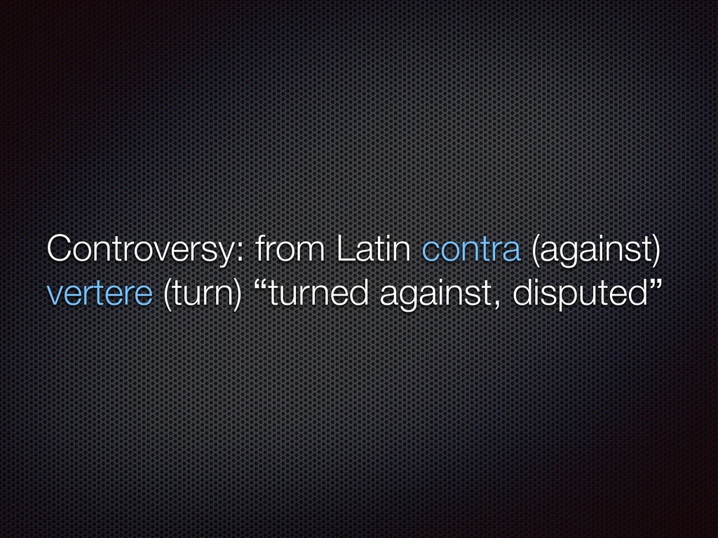
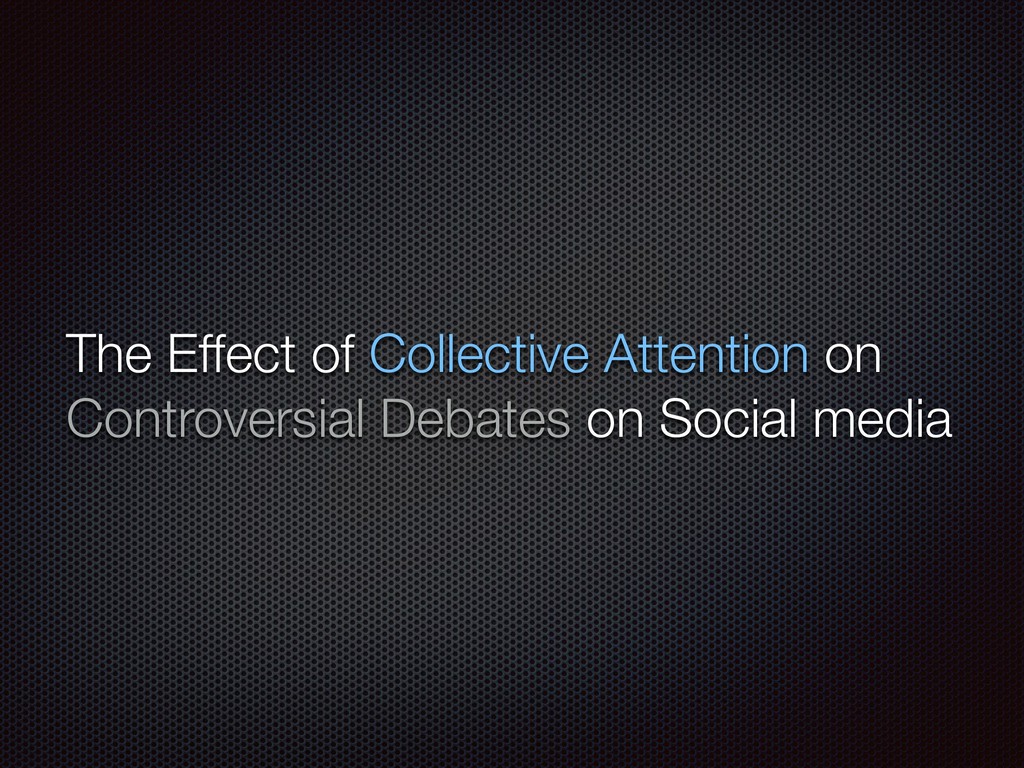
How do we discuss controversial topics on social media? 
Answering this question is not only interesting from a societal point of view, but also has concrete implications for policy makers, news agencies, and internet companies.
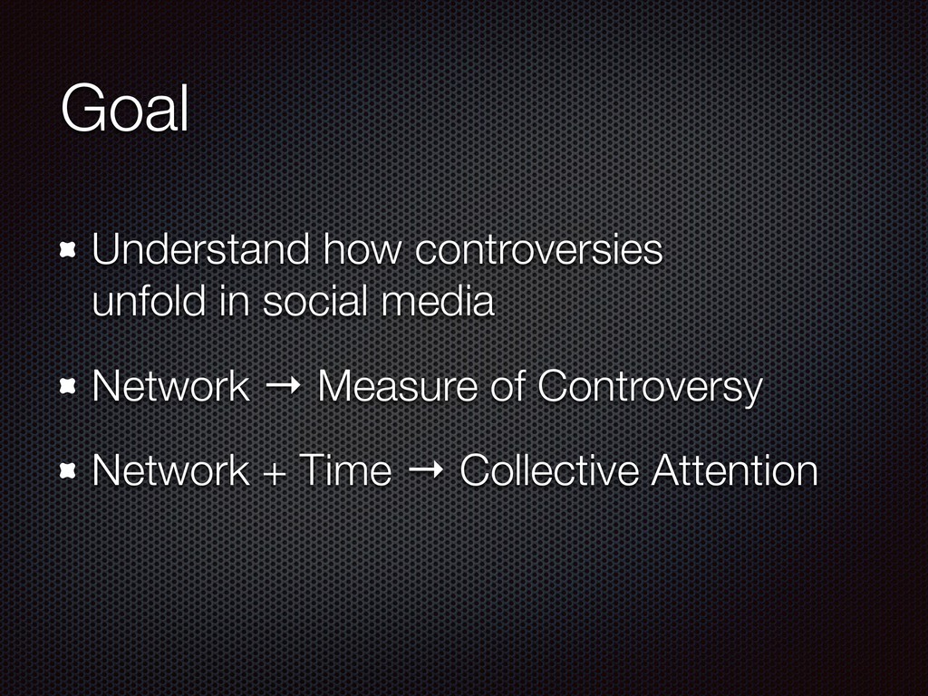
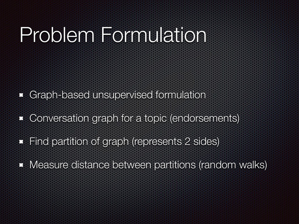
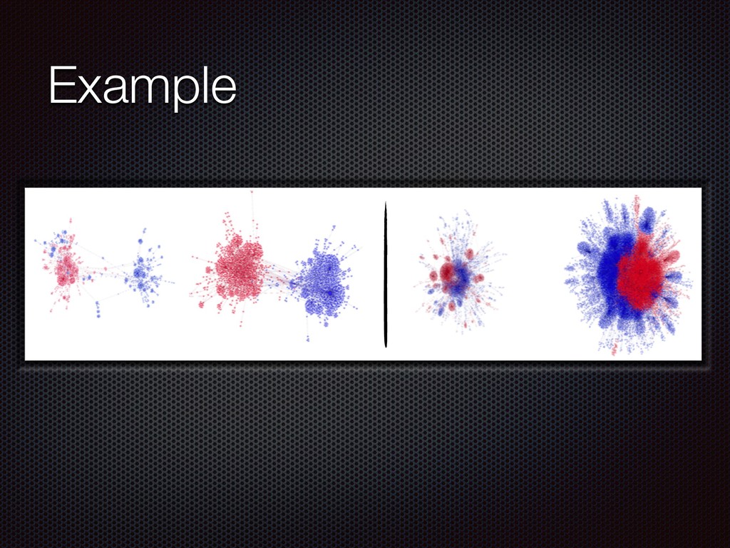
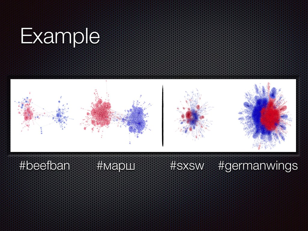
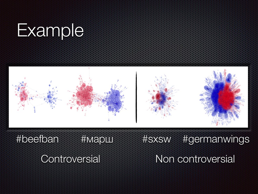
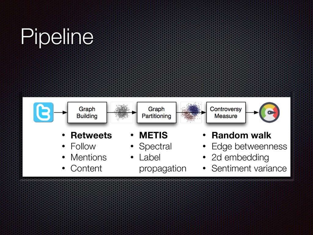
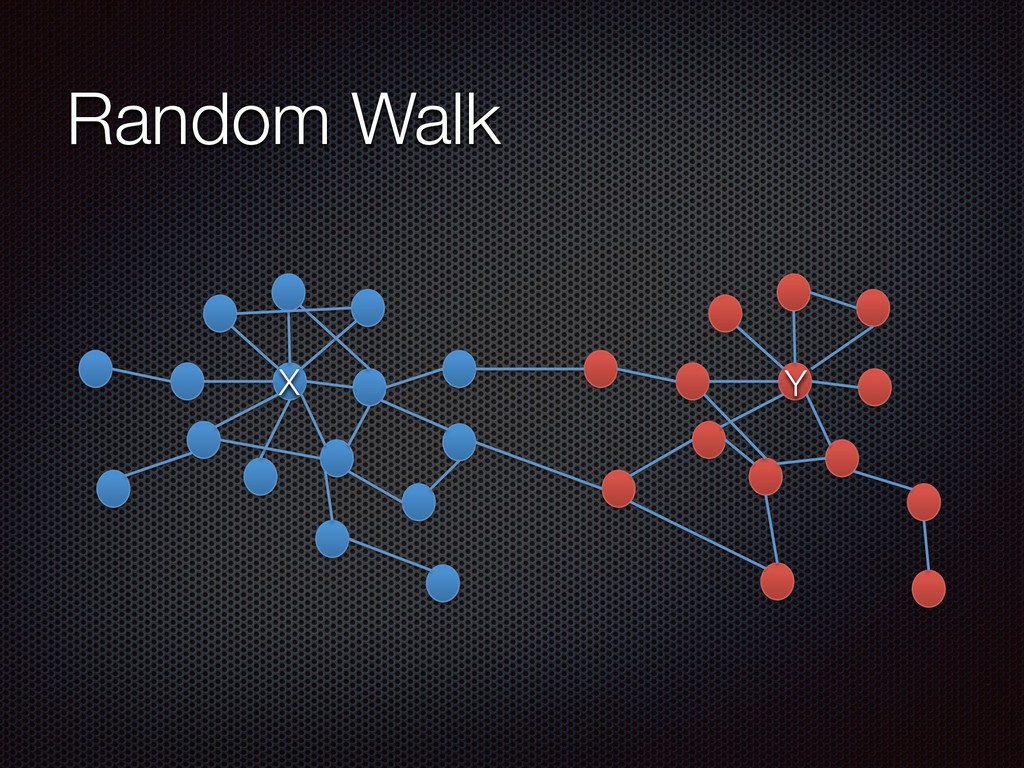
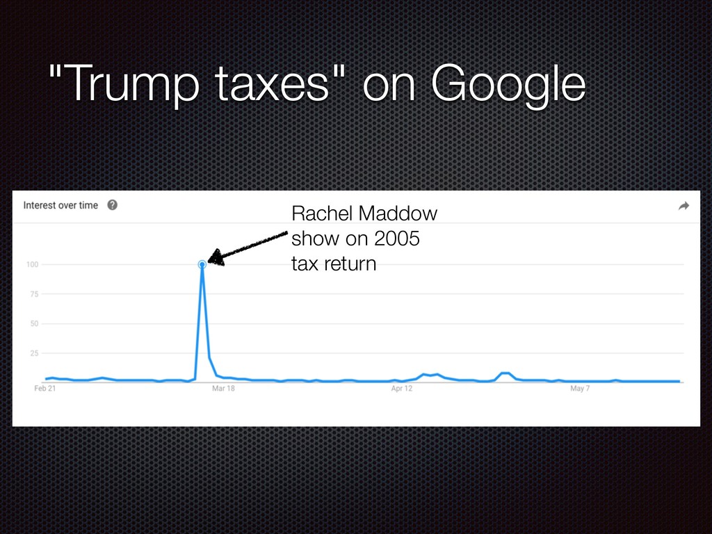
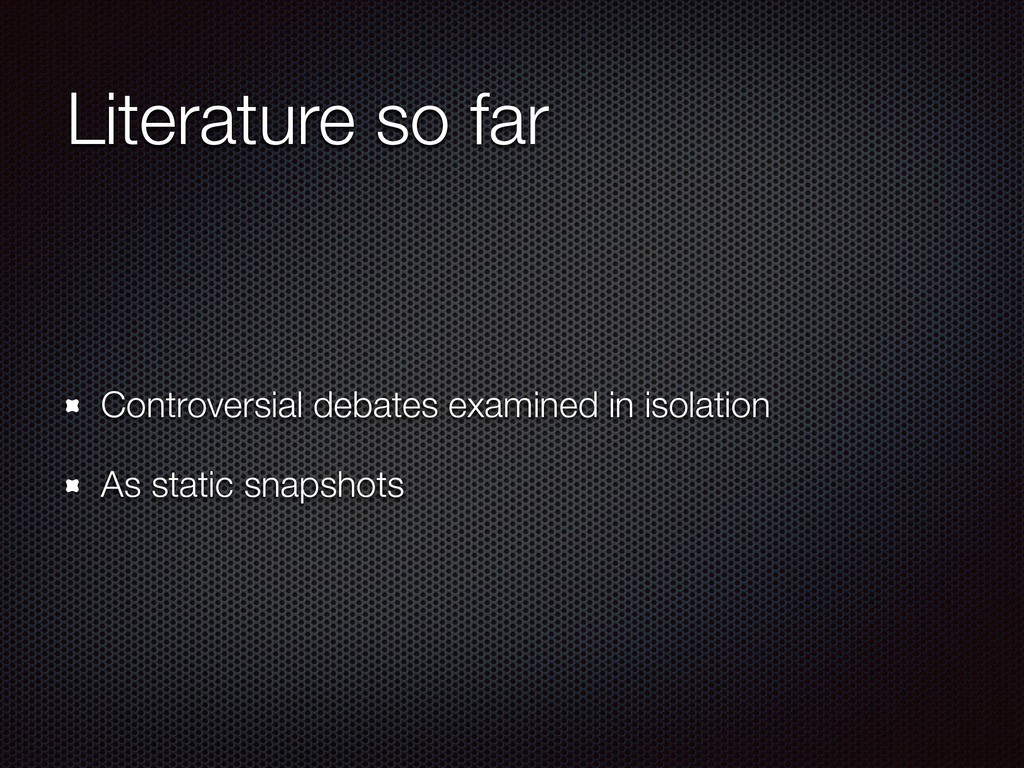
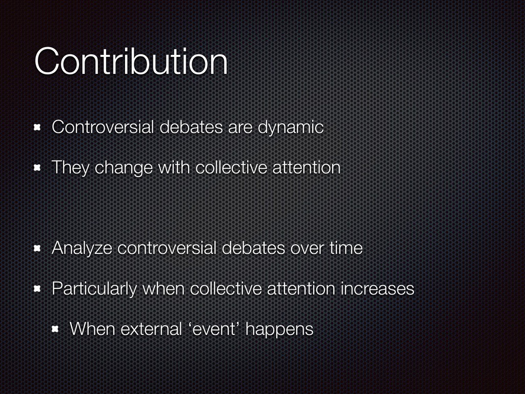
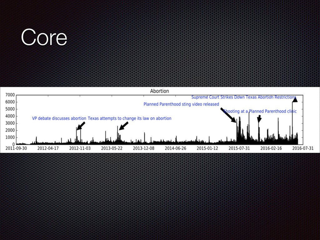
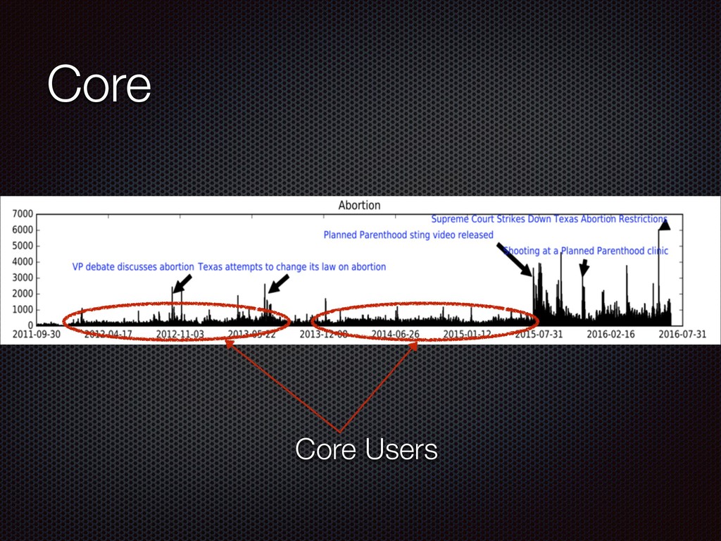
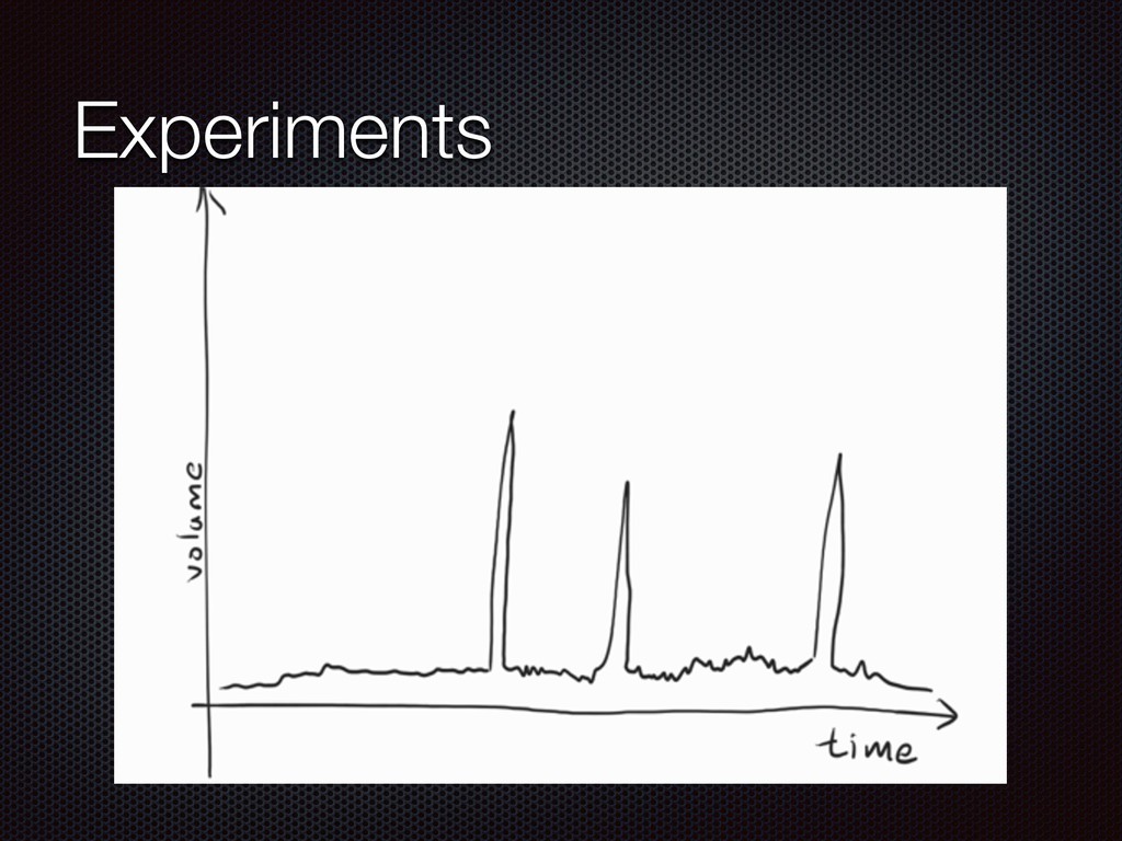
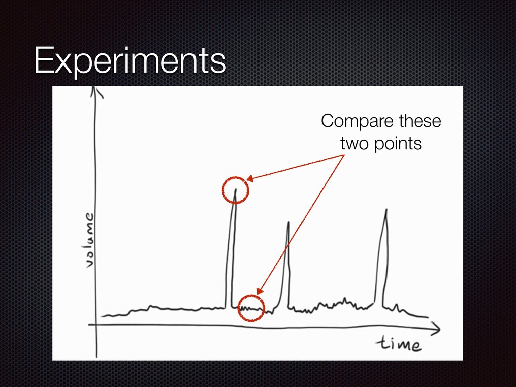
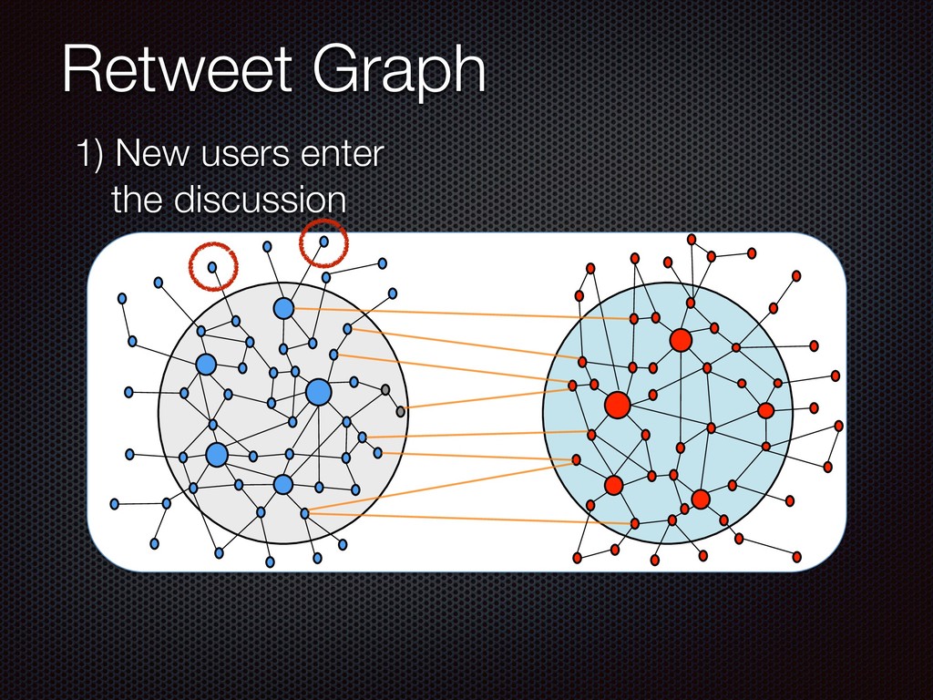
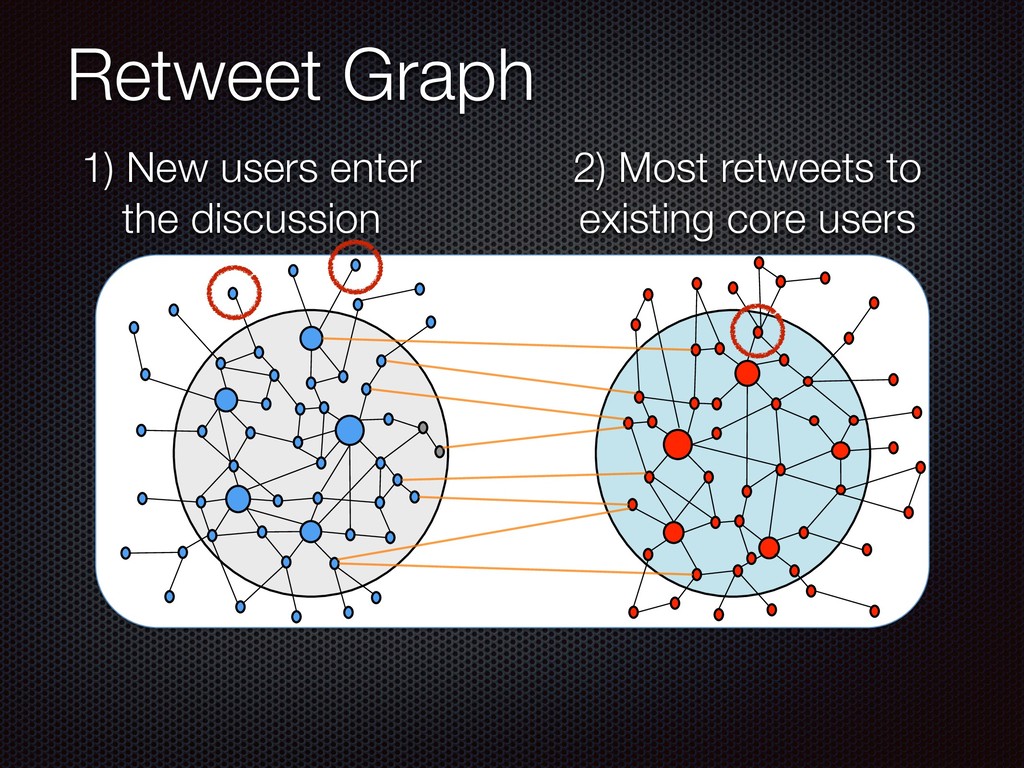
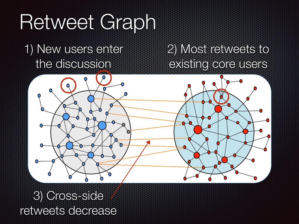
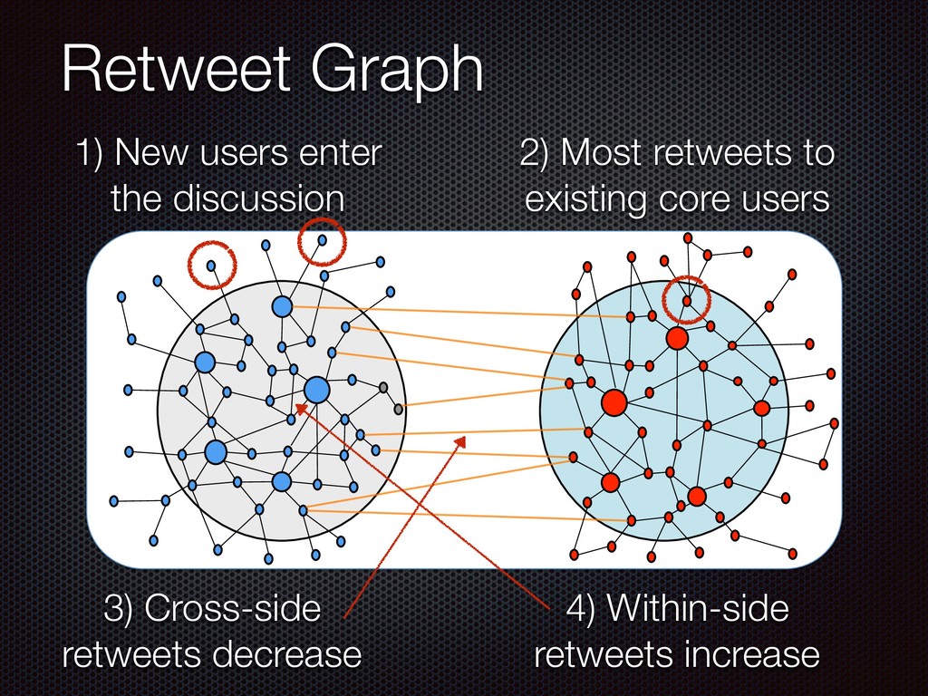
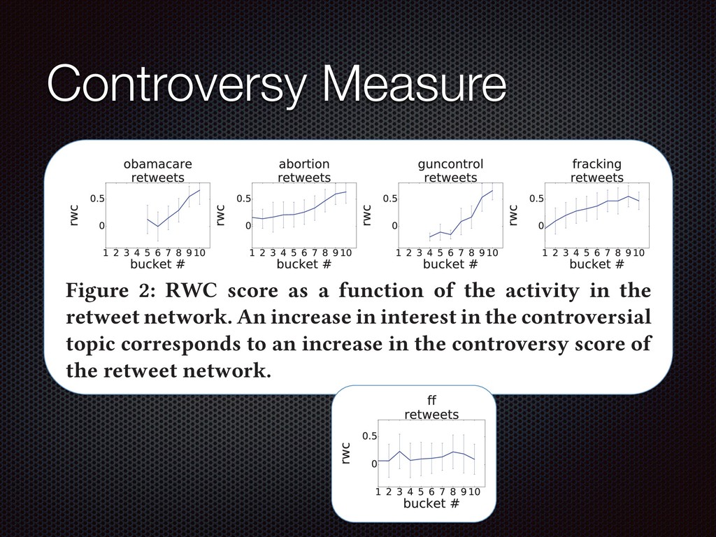
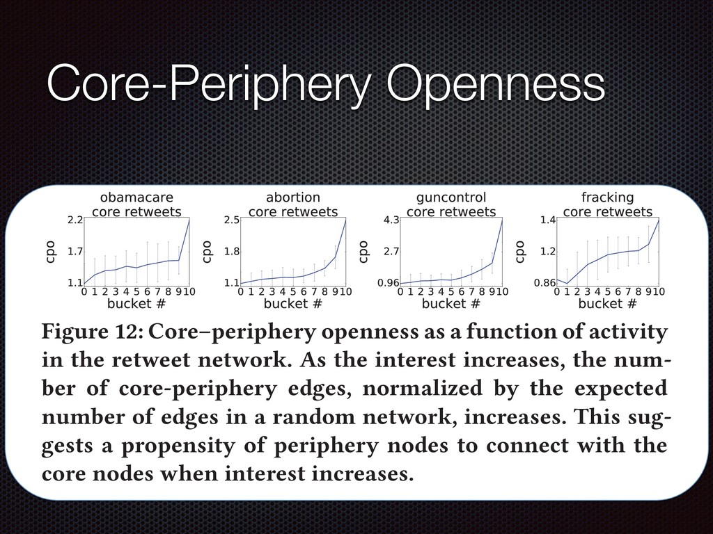
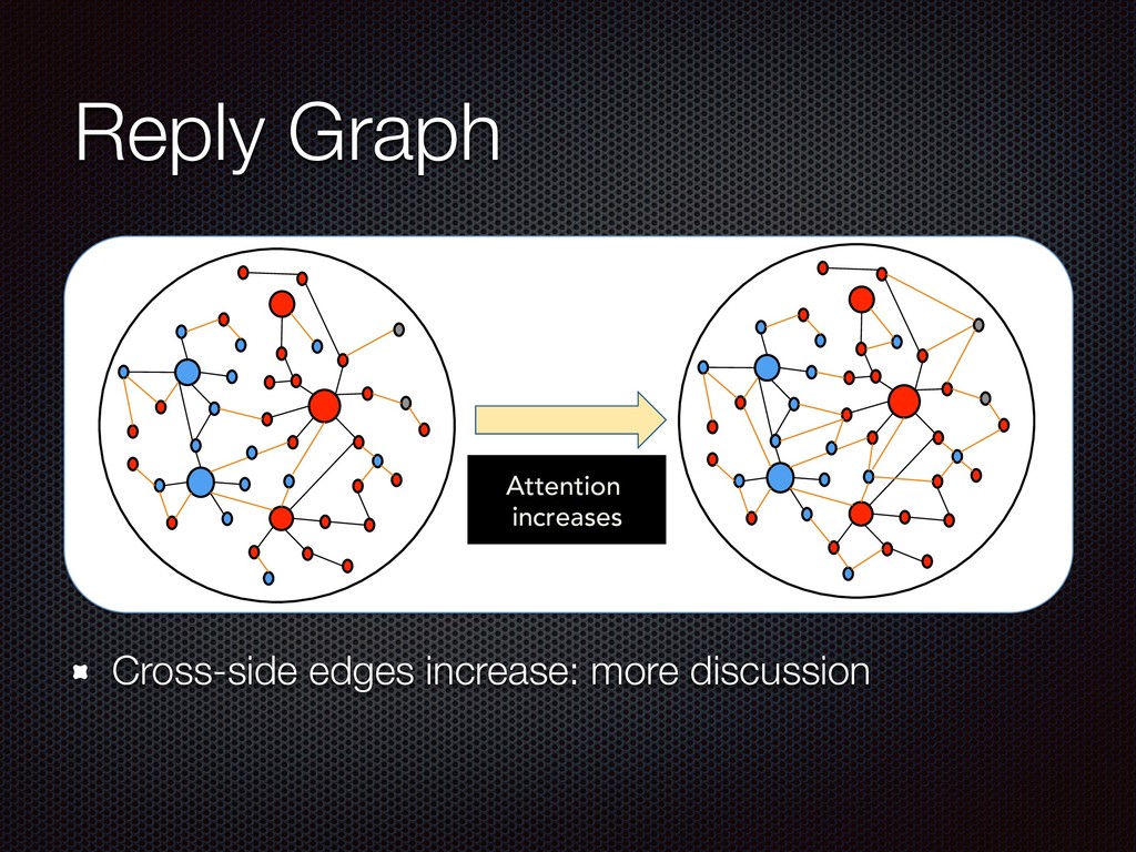
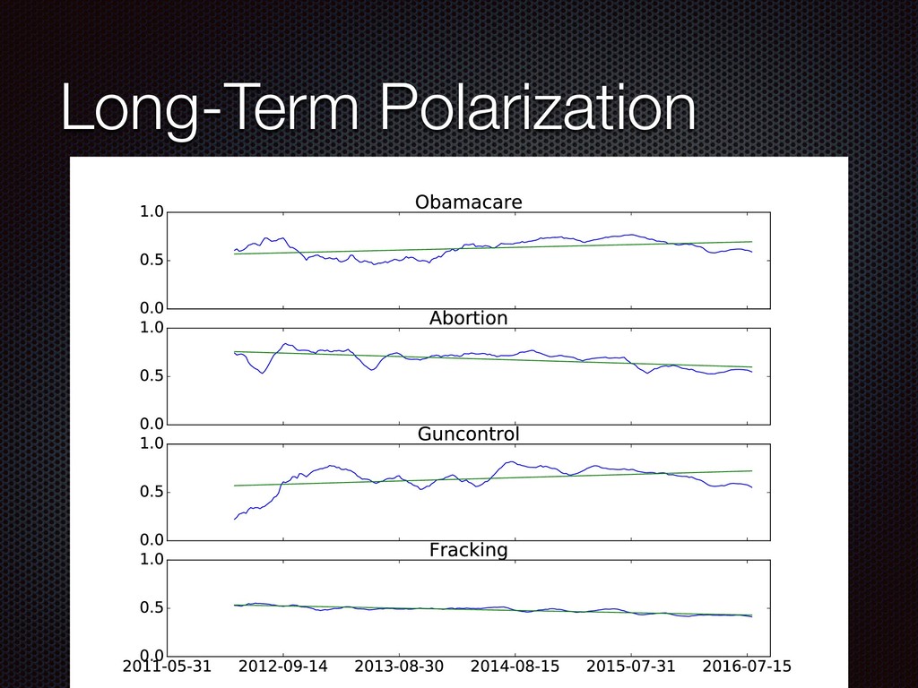
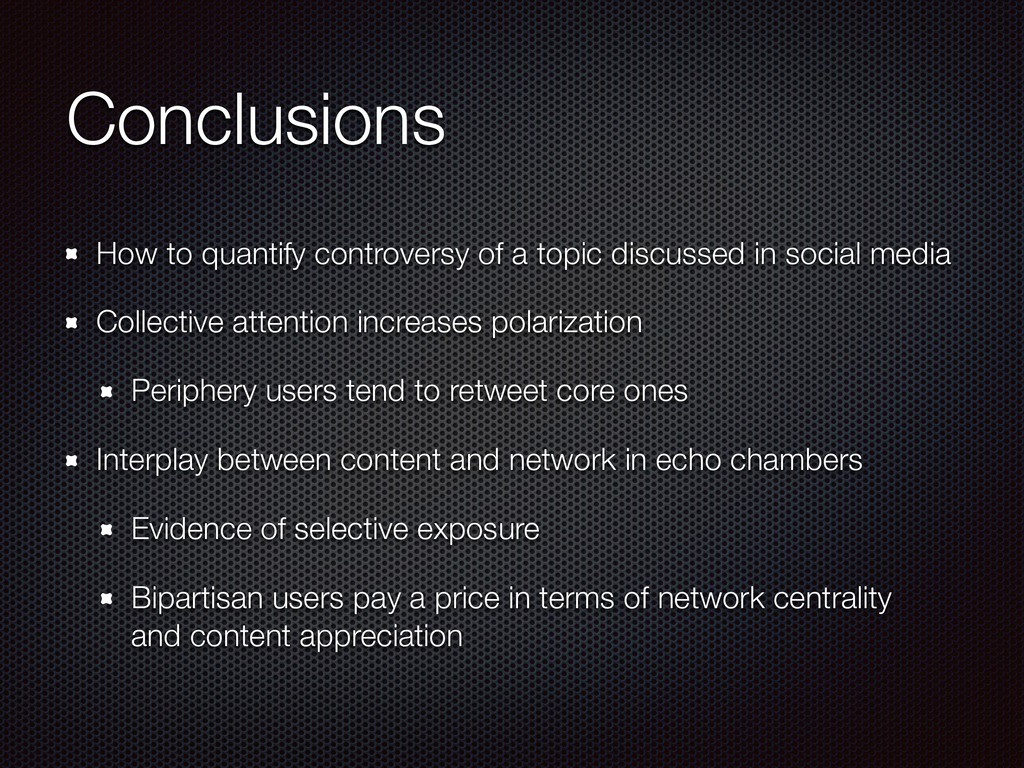
In this talk, we first take a look at how collective attention, which is typically related to external events that increase the visibility of the topic, changes the debate. Our analysis shows that, in long-lived controversial debates on Twitter, increased collective attention is associated with increased network polarization.
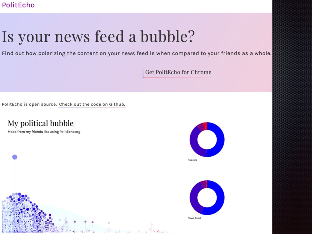
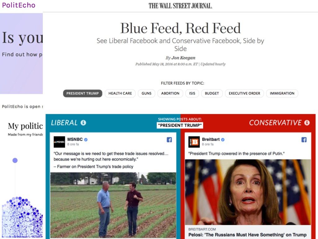
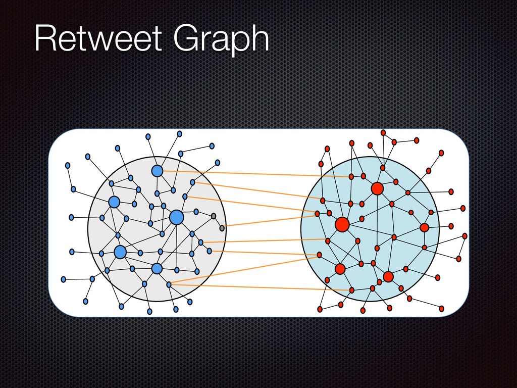
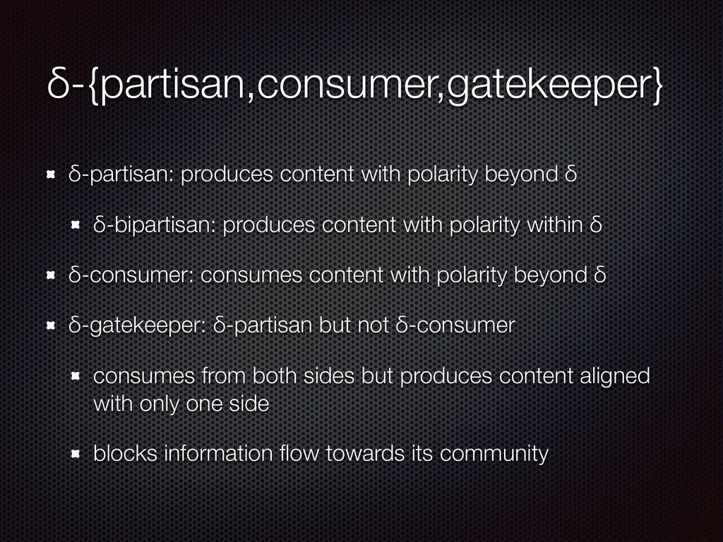
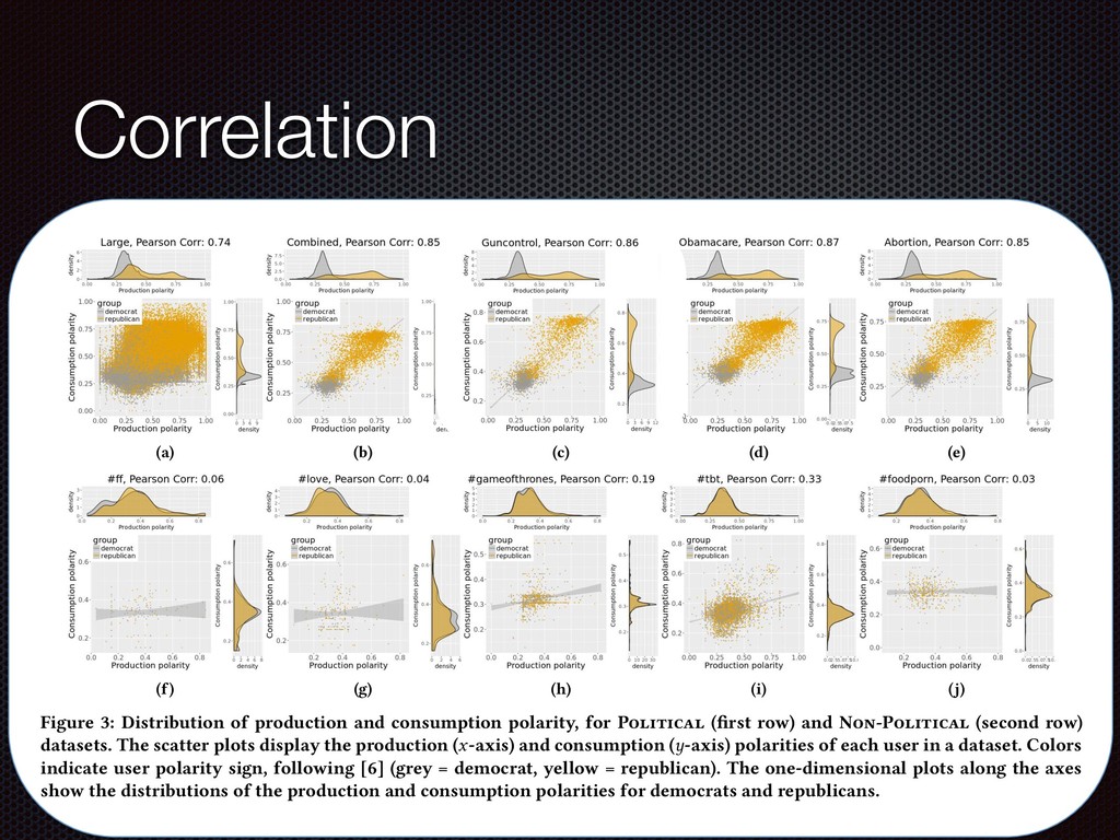
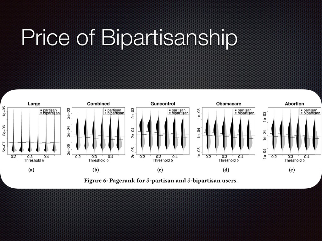
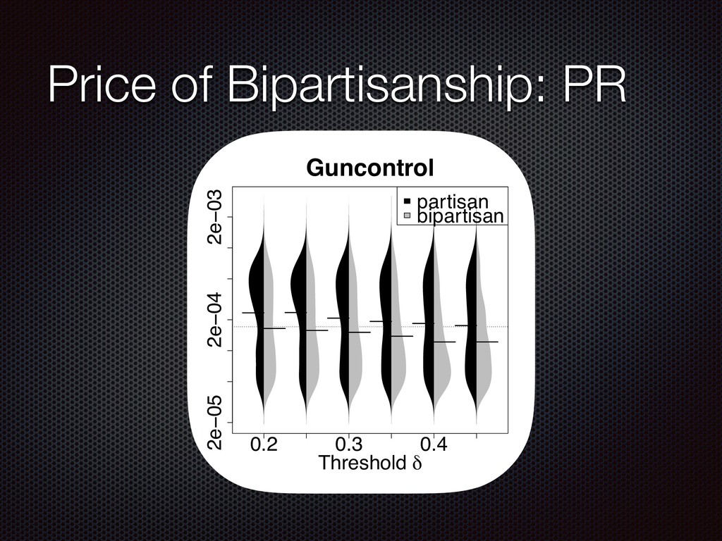
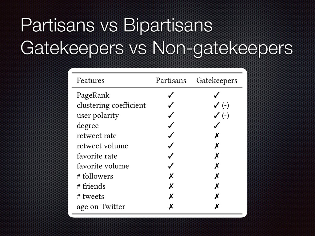
Then, we show how content and network interact in the formation of echo chambers. As expected, Twitter users are mostly exposed to political opinions that agree with their own. In addition, users who try to bridge the echo chambers by sharing content with diverse leaning have to pay a “price of bipartisanship” in terms of their network centrality and content appreciation.

Transcript

1. Controversy on Social Media:
   Collective Attention, Echo Chambers,
   and Price of Bipartisanship
   Gianmarco De Francisci Morales
   ISI Foundation
   with

   Kiran Garimella

   Aristides Gionis 

   Michael Mathioudakis
   

   View Slide

2. Controversy: from Latin contra (against)
   vertere (turn) “turned against, disputed”
   

   View Slide

3. View Slide

4. View Slide

5. View Slide

6. View Slide

7. There are two sides to every story
   

   View Slide

8. View Slide

9. View Slide

10. View Slide

11. Goal
    

    View Slide

12. Goal
    Understand how controversies 

    unfold in social media
    

    View Slide

13. Goal
    Understand how controversies 

    unfold in social media
    Network → Measure of Controversy
    

    View Slide

14. Goal
    Understand how controversies 

    unfold in social media
    Network → Measure of Controversy
    Network + Time → Collective Attention
    

    View Slide

15. Goal
    Understand how controversies 

    unfold in social media
    Network → Measure of Controversy
    Network + Time → Collective Attention
    Network + Content → Echo Chambers
    

    View Slide

16. Quantifying Controversy

    in Social Media 

    

    WSDM 2016
    

    View Slide

17. Black/Blue or White/Gold?
    

    View Slide

18. Desiderata
    In the wild
    Not necessarily political
    No domain knowledge
    Language independent
    Allows comparison
    

    View Slide

19. Problem Formulation
    Graph-based unsupervised formulation
    Conversation graph for a topic (endorsements)
    Find partition of graph (represents 2 sides)
    Measure distance between partitions (random walks)
    

    View Slide

20. Example
    

    View Slide

21. Example
    #beefban #марш #sxsw #germanwings
    

    View Slide

22. Example
    #beefban #марш #sxsw #germanwings
    Controversial Non controversial
    

    View Slide

23. Pipeline
    • Retweets
    • Follow
    • Mentions
    • Content
    • METIS
    • Spectral
    • Label 

    propagation
    • Random walk
    • Edge betweenness
    • 2d embedding
    • Sentiment variance
    

    View Slide

24. Random Walk
    

    View Slide

25. Random Walk
    X Y
    

    View Slide

26. Random Walk
    X Y
    

    View Slide

27. Controversy Detection
    

    View Slide

28. The Effect of Collective Attention on
    Controversial Debates on Social media

    

    WebSci 2017 (Best Paper Award)
    

    View Slide

29. The Effect of Collective Attention on
    Controversial Debates on Social media
    

    View Slide

30. The Effect of Collective Attention on
    Controversial Debates on Social media
    

    View Slide

31. The Effect of Collective Attention on
    Controversial Debates on Social media
    

    View Slide

32. The Effect of Collective Attention on
    Controversial Debates on Social media
    

    View Slide

33. "Trump taxes" on Google
    

    View Slide

34. "Trump taxes" on Google
    Rachel Maddow
    show on 2005
    tax return
    

    View Slide

35. Obamacare on Twitter
    

    View Slide

36. Gun Control on Twitter
    

    View Slide

37. Literature so far
    Controversial debates examined in isolation
    As static snapshots
    

    View Slide

38. Contribution
    Controversial debates are dynamic
    They change with collective attention
    Analyze controversial debates over time
    Particularly when collective attention increases
    When external ‘event’ happens
    

    View Slide

39. Data
    Twitter
    4 longitudinal polarized topics
    Obamacare, Abortion, Gun control, Fracking
    5 years (2011 -- 2016)
    Hundreds of thousands of users
    Millions of tweets
    

    View Slide

40. Definitions
    Retweet Graph
    Reply Graph
    Core Users
    

    View Slide

41. Retweet Graph
    

    View Slide

42. Reply graph
    

    View Slide

43. Core
    

    View Slide

44. Core
    Core Users
    

    View Slide

45. Experiments
    

    View Slide

46. Experiments
    Compare these

    two points
    

    View Slide

47. Retweet Graph
    

    View Slide

48. Retweet Graph
    1) New users enter
    the discussion
    

    View Slide

49. Retweet Graph
    2) Most retweets to
    existing core users
    1) New users enter
    the discussion
    

    View Slide

50. Retweet Graph
    2) Most retweets to
    existing core users
    1) New users enter
    the discussion
    3) Cross-side
    retweets decrease
    

    View Slide

51. Retweet Graph
    2) Most retweets to
    existing core users
    1) New users enter
    the discussion
    3) Cross-side
    retweets decrease
    4) Within-side
    retweets increase
    

    View Slide

52. Controversy Measure
    Figure 2: RWC score as a function of the activity in the
    retweet network. An increase in interest in the controversial
    topic corresponds to an increase in the controversy score of
    the retweet network.
    5.1 Network
    F
    t
    r
    s
    w
    

    View Slide

53. Core-Periphery Openness
    Figure 12: Core–periphery openness as a function of activity
    in the retweet network. As the interest increases, the num-
    ber of core-periphery edges, normalized by the expected
    number of edges in a random network, increases. This sug-
    gests a propensity of periphery nodes to connect with the
    core nodes when interest increases.
    

    View Slide

54. Reply Graph
    Cross-side edges increase: more discussion
    Attention
    increases
    

    View Slide

55. Content
    Pro Life
    Pro Choice
    Normal

    Condition
    Attention

    Increase
    

    View Slide

56. Content
    Pro Life
    Pro Choice
    Normal

    Condition
    Attention

    Increase
    Content becomes uniform across the sides
    

    View Slide

57. Long-Term Polarization
    

    View Slide

58. Summary
    Controversial debates during external events
    Polarization increases
    Retweet graph becomes hierarchical (core-periphery)
    More replies across sides
    Content becomes more uniform
    Many more results in the paper!
    

    View Slide

59. Political Discourse on Social Media
    Echo Chambers, Gatekeepers, 

    and the Price of Bipartisanship
    WWW 2018
    

    View Slide

60. Political Discourse on

    Social Media
    Characterized by heavy polarization
    Emergence of echo chambers ("Hear your own voice")
    Might hamper deliberative process in democracy
    Lack of shared world view
    Concern expressed by former US Presidents,
    Facebook, Twitter, and more
    

    View Slide

61. Polarization Cause
    Selective exposure?
    People see only content that agrees with their pre-
    existing opinion
    Biased assimilation?
    People pay more attention to content that agrees
    with their pre-existing opinion
    

    View Slide

62. Echo Chamber Definition
    Echo = opinion
    Chamber = network
    Joint content + network definition
    Echo chamber = political leaning of content that users
    receive from network agrees with that of content they
    share to the network
    

    View Slide

63. Production/Consumption
    Consumption
    What you receive in your feed
    What your followees tweet
    Production
    What you tweet
    

    View Slide

64. Political Leaning Scores
    Based on source of the content (500 domains)
    Score derived by self-declared affiliation of sharers on FB
    FoxNews.com is aligned with conservatives (CP = 0.9),

    HuffingtonPost.com is aligned with liberals (CP = 0.17)
    

    View Slide

65. Production/Consumption
    Scores
    Polarity scores based on “content” leaning (from source)
    Production score
    Average political leaning of the content the user tweets
    Consumption score
    Average political leaning of the content the user receives on
    their feed
    Results of selection by the user
    

    View Slide

66. δ-partisanship
    f
    s
    n-
    r
    e
    m-
    .,
    s
    n
    e
    e
    k
    Figure 1: Example showing the denition of -partisan users.
    The dotted red lines are drawn at and 1- . Users on the left
    of the leftmost dashed red line or right of the rightmost one
    are -partisan.
    

    View Slide

67. δ-{partisan,consumer,gatekeeper}
    δ-partisan: produces content with polarity beyond δ
    δ-bipartisan: produces content with polarity within δ
    δ-consumer: consumes content with polarity beyond δ
    δ-gatekeeper: δ-partisan but not δ-consumer
    consumes from both sides but produces content aligned
    with only one side
    blocks information flow towards its community
    

    View Slide

68. Network Measures
    Network-based latent-space user polarity
    Based on following politicians with aligned ideology
    Network centrality (PageRank)
    Local clustering coefficient
    Retweet/favorite rates and volumes
    

    View Slide

69. (a) (b) (c) (d) (e)
    (f) (g) (h) (i) (j)
    Figure 3: Distribution of production and consumption polarity, for P (rst row) and NP (second row)
    datasets. The scatter plots display the production (
    x
    -axis) and consumption ( -axis) polarities of each user in a dataset. Colors
    indicate user polarity sign, following [6] (grey = democrat, yellow = republican). The one-dimensional plots along the axes
    show the distributions of the production and consumption polarities for democrats and republicans.
    Correlation
    (a) (b) (c) (d) (e)
    (f) (g) (h) (i) (j)
    Figure 3: Distribution of production and consumption polarity, for P (rst row) and NP (second row)
    datasets. The scatter plots display the production (
    x
    -axis) and consumption ( -axis) polarities of each user in a dataset. Colors
    indicate user polarity sign, following [6] (grey = democrat, yellow = republican). The one-dimensional plots along the axes
    show the distributions of the production and consumption polarities for democrats and republicans.
    

    View Slide

70. Correlation: Gun Control
    

    View Slide

71. (f) (g) (h) (i) (j)
    Figure 3: Distribution of production and consumption polarity, for P (rst row) and NP (second row)
    datasets. The scatter plots display the production (
    x
    -axis) and consumption ( -axis) polarities of each user in a dataset. Colors
    indicate user polarity sign, following [6] (grey = democrat, yellow = republican). The one-dimensional plots along the axes
    show the distributions of the production and consumption polarities for democrats and republicans.
    (a) (b) (c) (d) (e)
    (f) (g) (h) (i) (j)
    Figure 4: Top: Production polarity variance vs. production polarity (mean). Bottom: Consumption polarity variance vs. con-
    sumption polarity (mean).
    However, dierently from the rest of the side they align with, they
    show a lower clustering coecient, an indication that they are
    not completely embedded in a single community. Given that they
    receive content also from the opposing side, this result is to be
    Finally, given that both partisans and gatekeepers sport higher
    centrality, we compare their PageRank values directly and nd that
    there is a signicant dierence: partisans have a higher PageRank
    compared to gatekeepers (gure not shown). This eect is more
    Variance
    (f) (g) (h) (i) (j)
    Figure 3: Distribution of production and consumption polarity, for P (rst row) and NP (second row)
    datasets. The scatter plots display the production (
    x
    -axis) and consumption ( -axis) polarities of each user in a dataset. Colors
    indicate user polarity sign, following [6] (grey = democrat, yellow = republican). The one-dimensional plots along the axes
    show the distributions of the production and consumption polarities for democrats and republicans.
    (a) (b) (c) (d) (e)
    (f) (g) (h) (i) (j)
    Figure 4: Top: Production polarity variance vs. production polarity (mean). Bottom: Consumption polarity variance vs. con-
    sumption polarity (mean).
    However, dierently from the rest of the side they align with, they
    show a lower clustering coecient, an indication that they are
    not completely embedded in a single community. Given that they
    receive content also from the opposing side, this result is to be
    Finally, given that both partisans and gatekeepers sport higher
    centrality, we compare their PageRank values directly and nd that
    there is a signicant dierence: partisans have a higher PageRank
    compared to gatekeepers (gure not shown). This eect is more
    

    View Slide

72. Variance
    (b) (c)
    

    View Slide

73. 0.0 1.0 2.0
    0.2 0.3 0.4
    Large
    Threshold δ
    partisan
    bipartisan
    (a)
    0.0 1.0 2.0
    0.2 0.3 0.4
    Combined
    Threshold δ
    partisan
    bipartisan
    (b)
    −0.5 0.5 1.5 2.5
    0.2 0.3 0.4
    Guncontrol
    Threshold δ
    partisan
    bipartisan
    (c)
    0.0 1.0 2.0
    0.2 0.3 0.4
    Obamacare
    Threshold δ
    partisan
    bipartisan
    (d)
    0.0 1.0 2.0
    0.2 0.3 0.4
    Abortion
    Threshold δ
    partisan
    bipartisan
    (e)
    Figure 5: Absolute value of the user polarity scores for -partisan and -bipartisan users.
    5e−07 2e−06 1e−05
    0.2 0.3 0.4
    Large
    Threshold δ
    partisan
    bipartisan
    (a)
    2e−05 2e−04 2e−03
    0.2 0.3 0.4
    Combined
    Threshold δ
    partisan
    bipartisan
    (b)
    2e−05 2e−04 2e−03
    0.2 0.3 0.4
    Guncontrol
    Threshold δ
    partisan
    bipartisan
    (c)
    1e−05 1e−04 1e−03
    0.2 0.3 0.4
    Obamacare
    Threshold δ
    partisan
    bipartisan
    (d)
    1e−05 1e−04 1e−03
    0.2 0.3 0.4
    Abortion
    Threshold δ
    partisan
    bipartisan
    (e)
    Figure 6: Pagerank for -partisan and -bipartisan users.
    ble 3: Comparison between -gatekeeper users and a ran-
    m sample of normal users. A 3 indicates that the corre-
    onding property is signicantly higher for gatekeepers
    < 0.001) for at least 4 of the 6 thresholds used. A mi-
    s next to the checkmark (-) indicates that the property is
    nicantly lower.
    Table 4: Accuracy for prediction of users who are pa
    sans (
    p
    ) or gatekeepers ( ). (net) indicates network and p
    le features only, (
    n
    -gram) indicates just n-gram featur
    The last two columns show results for all features combin
    p (net) (net) p (n-gram) (n-gram) p
    Price of Bipartisanship
    0.0 1.0 2.0
    0.2 0.3 0.4
    Large
    Threshold δ
    partisan
    bipartisan
    (a)
    0.0 1.0 2.0
    0.2 0.3 0.4
    Combined
    Threshold δ
    partisan
    bipartisan
    (b)
    −0.5 0.5 1.5 2.5
    0.2 0.3 0.4
    Guncontrol
    Threshold δ
    partisan
    bipartisan
    (c)
    0.0 1.0 2.0
    0.2 0.3 0.4
    Obamacare
    Threshold δ
    partisan
    bipartisan
    (d)
    0.0 1.0 2.0
    0.2 0.3 0.4
    Abortion
    Threshold δ
    partisan
    bipartisan
    (e)
    Figure 5: Absolute value of the user polarity scores for -partisan and -bipartisan users.
    5e−07 2e−06 1e−05
    0.2 0.3 0.4
    Large
    Threshold δ
    partisan
    bipartisan
    (a)
    2e−05 2e−04 2e−03
    0.2 0.3 0.4
    Combined
    Threshold δ
    partisan
    bipartisan
    (b)
    2e−05 2e−04 2e−03
    0.2 0.3 0.4
    Guncontrol
    Threshold δ
    partisan
    bipartisan
    (c)
    1e−05 1e−04 1e−03
    0.2 0.3 0.4
    Obamacare
    Threshold δ
    partisan
    bipartisan
    (d)
    1e−05 1e−04 1e−03
    0.2 0.3 0.4
    Abortion
    Threshold δ
    partisan
    bipartisan
    (e)
    Figure 6: Pagerank for -partisan and -bipartisan users.
    ble 3: Comparison between -gatekeeper users and a ran-
    m sample of normal users. A 3 indicates that the corre-
    onding property is signicantly higher for gatekeepers
    < 0.001) for at least 4 of the 6 thresholds used. A mi-
    s next to the checkmark (-) indicates that the property is
    nicantly lower.
    Table 4: Accuracy for prediction of users who are pa
    sans (
    p
    ) or gatekeepers ( ). (net) indicates network and p
    le features only, (
    n
    -gram) indicates just n-gram featur
    The last two columns show results for all features combin
    p (net) (net) p (n-gram) (n-gram) p
    

    View Slide

74. Price of Bipartisanship: PR
    hreshold δ
    (b)
    Threshold δ
    (c)
    Thresh
    (d)
    value of the user polarity scores for -partisan and
    0.3 0.4
    ombined
    hreshold δ
    partisan
    bipartisan
    (b)
    2e−05 2e−04 2e−03
    0.2 0.3 0.4
    Guncontrol
    Threshold δ
    partisan
    bipartisan
    (c)
    1e−05 1e−04 1e−03
    0.2 0.3
    Obama
    Thresh
    (d)
    

    View Slide

75. Partisans vs Bipartisans

    Gatekeepers vs Non-gatekeepers
    ons
    d of
    g of
    pro-
    urce
    pro-
    the
    and
    ddi-
    for
    ties.
    (for
    and
    mp-
    also
    pro-
    rces.
    ach
    The
    Table 2: Comparison of various features for partisans & bi-
    partisans and gatekeepers & non-gatekeepers. A 3 indicates
    that the corresponding feature is signicantly higher for the
    group of the column (
    p
    < 0.001) for at least 4 of the 6 thresh-
    olds used, for most datasets. A minus next to the check-
    mark (-) indicates that the feature is signicantly lower.
    Features Partisans Gatekeepers
    PageRank 3 3
    clustering coecient 3 (-) 3 (-)
    user polarity 3 (-) 3 (-)
    degree 3 3
    retweet rate 3 7
    retweet volume 3 7
    favorite rate 3 7
    favorite volume 3 7
    # followers 7 7
    # friends 7 7
    # tweets 7 7
    age on Twitter 7 7
    datasets).9 A “3 (-)” means that the property is signicantly lower
    

    View Slide

76. Conclusions
    How to quantify controversy of a topic discussed in social media
    Collective attention increases polarization
    Periphery users tend to retweet core ones
    Interplay between content and network in echo chambers
    Evidence of selective exposure
    Bipartisan users pay a price in terms of network centrality 

    and content appreciation
    

    View Slide

77. What's next?
    Joint opinion formation + network generation model
    Temporal dynamics of the process
    Application to other contexts (Reddit, Facebook)
    Interventions: can we do something about it?
    

    View Slide

78. Thanks!
    Ask me two questions!
    56
    @gdfm7
    gdfm@acm.org
    

    View Slide