Quantifying and Reducing Controversy in Social Media

Transcript

1. Quantifying and Reducing
   Controversy in Social Media
   Gianmarco De Francisci Morales
   

   with Kiran Garimella, Aristides Gionis, Michael Mathioudakis
   

   View Slide

2. Controversy: from Latin contra (against)
   vertere (turn) “turned against, disputed”
   

   View Slide

3. View Slide

4. View Slide

5. View Slide

6. There are two sides to every story
   

   View Slide

7. The gap grows
   

   View Slide

8. The gap grows
   

   View Slide

9. Goal
   Detect and quantify controversies automatically
   Use social media data as sensors
   Design methods to reduce controversy
   By exposing people to contrarian points of view
   

   View Slide

10. Quantifying Controversy
    In the wild
    Not necessarily political
    

    View Slide

11. Black/Blue or White/Gold?
    

    View Slide

12. Quantifying Controversy
    In the wild
    Not necessarily political
    No domain knowledge
    Language independent
    Allows comparison
    

    View Slide

13. Problem Formulation
    Graph-based unsupervised formulation
    Conversation graph for a topic (posts, endorsements)
    Find partition of graph (represents 2 sides)
    Measure distance between partitions (random walks)
    

    View Slide

14. Example
    

    View Slide

15. Example
    #beefban #марш #sxsw #germanwings
    

    View Slide

16. Example
    #beefban #марш #sxsw #germanwings
    Controversial Non controversial
    

    View Slide

17. Pipeline
    • Retweets
    • Follow
    • Mentions
    • Content
    • METIS
    • Spectral
    • Label 

    propagation
    • Random walk
    • Edge betweenness
    • 2d embedding
    • Sentiment variance
    

    View Slide

18. Single #hashtag is not sufficient
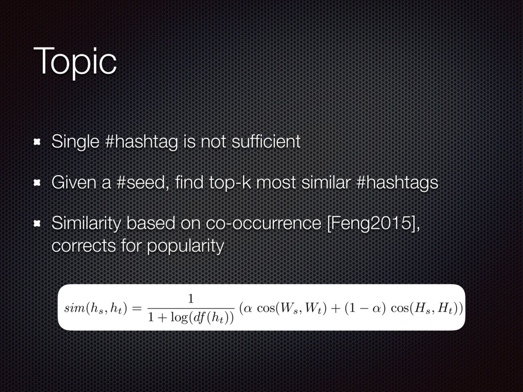
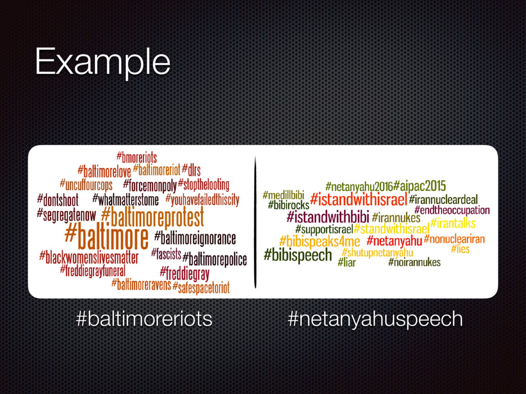
    Given a #seed, find top-k most similar #hashtags
    Similarity based on co-occurrence [Feng2015],
    corrects for popularity

    

    

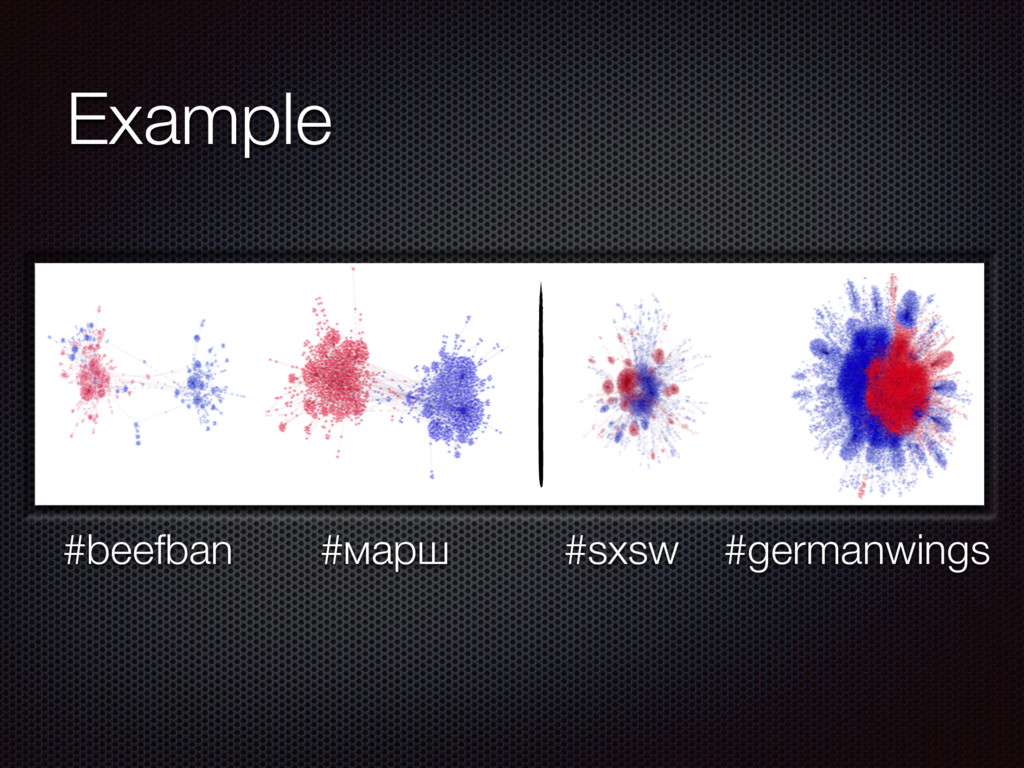
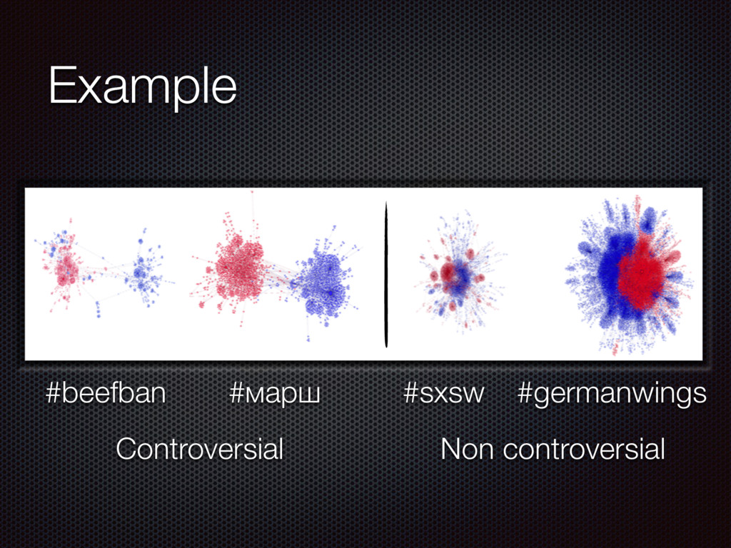
    Topic
    as a means to express their opinion. Using a single hashtag may thus miss part of th
    relevant posts.
    To address this limitation, we extend the definition of topic to be more encompassin
    Given a seed hashtag, we define a topic as a set of related hashtags, which co-occur wit
    the seed hashtag. To find related hashtags, we employ (and improve upon) a recen
    clustering algorithm tailored for the purpose [Feng et al. 2015].
    Feng et al. [2015] develop a simple measure to compute the similarity between tw
    hashtags, which relies on co-occurring words and hashtags. The authors then use th
    similarity measure to find closely related hashtags and define clusters. However, th
    simple approach presents one drawback, in that very popular hashtags such as #ff o
    #follow co-occur with a large number of hashtags. Hence, directly applying the origina
    approach results in extremely noisy clusters. Since the quality of the topic affect
    critically the entire pipeline, we want to avert this issue and ensure minimal noise
    introduced in the expanded set of hashtags.
    Therefore, we improve the basic approach by taking into account and normalizin
    for the popularity of the hashtags. Specifically, we compute the document frequenc
    of all hashtags on a random 1% sample of the Twitter stream, and normalize th
    original similarity score between two hashtags by the inverse document frequency. Th
    similarity score is formally defined as
    sim
    (
    h
    s
    , h
    t) =
    1
    1 + log(
    df
    (
    h
    t))
    (
    ↵
    cos(
    W
    s
    , W
    t) + (1
    ↵
    ) cos(
    H
    s
    , H
    t))
    , (1
    where h
    s
    is the seed tag, h
    t
    is the candidate tag, W
    x
    and H
    x
    are the sets of word
    and hashtags that co-occur with hashtag h
    x
    , respectively,
    cos
    is the cosine similarit
    between two vectors, df is the document frequency of a tag, and ↵ is a parameter tha
    

    View Slide

19. Example
    A:7
    (a) (b)
    Fig. 2: Sets of related hashtags for the topics (a) #baltimoreriots and (b) #netanyahuspeech.
    4.2. Data aspects
    For each topic, we retrieve all tweets that contain one of its hashtags and that are
    generated during the observation window. We also ensure that the selected hashtags
    #baltimoreriots #netanyahuspeech
    

    View Slide

20. Endorsement Graph
    Topic specific
    Vertex = user
    Edge = endorsement for the topic
    At least τ retweets
    

    View Slide

21. A:9
    (a) (b) (c) (d)
    (e) (f) (g) (h)
    Fig. 3: Sample conversation graphs with retweet (top) and follow (bottom) aspects (visualized
    using the force-directed layout algorithm in Gephi). The left side is controversial, (a,e) #beefban,
    (b,f) #russia march, while the right side is non-controversial, (c,g) #sxsw, (d,h) #germanwings.
    

    View Slide

22. RWC Rationale
    Random Walk Controversy score
    Zaller's RAS model (Receive, Accept, Sample) 

    "The Nature and Origins of Mass Opinion"
    Response Axiom: "Individuals form opinions by averaging across
    the considerations that are immediately salient or accessible to
    them"
    Authoritative (influential) users with high degree set opinions
    Measure likelihood a user to be exposed to opinions from influential
    users on either side
    

    View Slide

23. Random Walk
    

    View Slide

24. Random Walk
    

    View Slide

25. Random Walk
    X Y
    

    View Slide

26. Random Walk
    X Y
    

    View Slide

27. RWC Definition
    we select one partition at random (each with
    walk that starts from a random vertex in tha
    visits any high-degree vertex (from either sid
    dom Walk Controversy
    (RWC) measure as fo
    ending in partition X and one ending in par
    obabilities of two events: (i) both random wa
    in and (ii) both random walks started in a pa
    The measure is quantified as
    RWC
    =
    P
    XX
    P
    Y Y
    P
    Y X
    P
    XY
    ,
    X, Y
    }
    is the conditional probability
    AB =
    Pr
    [
    start in partition A
    |
    end in partition
    probabilities have the following desirable prop
    Consider two random walks, one ending in partition X and one ending in
    partition Y , RWC is the difference of the probabilities of two events: (i)
    both random walks started from the partition they ended in and (ii) both
    random walks started in a partition other than the one they ended in
    (a) (b)
    Partitions obtained for (a) #beefban, (b) #russia march by using the hybrid graph
    ch. The partitions are more noisy than those in Figures 3(a,b).
    Subsequently, we select one partition at random (each with probability
    0
    er a random walk that starts from a random vertex in that partition. Th
    nates when it visits any high-degree vertex (from either side).
    define the
    Random Walk Controversy
    (RWC) measure as follows. “Consi
    m walks, one ending in partition X and one ending in partition Y , RWC
    nce of the probabilities of two events: (i) both random walks started fr
    on they ended in and (ii) both random walks started in a partition other t
    ey ended in.” The measure is quantified as
    RWC
    =
    P
    XX
    P
    Y Y
    P
    Y X
    P
    XY
    ,
    P
    AB
    , A, B
    2 {
    X, Y
    }
    is the conditional probability
    P
    AB =
    Pr
    [
    start in partition A
    |
    end in partition B
    ]
    .
    orementioned probabilities have the following desirable properties: (i) they
    d by the size of each partition, as the random walk starts with equal pro
    ach partition, and (ii) they are not skewed by the total degree of vertices
    

    View Slide

28. RWC Properties
    Probabilities are conditional on ending in either partition
    Random walks end on either side with equal probability
    Not skewed by size of each partition
    Not skewed by total degree of vertices in each partition
    Close to 1 when probability of crossing sides low (high
    controversy)
    Close to 0 when probability of crossing comparable to that of
    staying (low controversy)
    

    View Slide

29. RWC Computation
    Monte Carlo sampling (slow)
    Efficient implementation as random walk with restart
    (RWR)
    As a byproduct, possible to compute polarization score
    for each user
    Expected hitting time for a user to an influencer
    

    View Slide

30. Datasets
    A:5
    Table I: Datasets statistics: hashtag, sizes of the follow and retweet graphs, and description
    of the event. The top group represent controversial topics, while the bottom one represent
    non-controversial ones.
    Hashtag # Tweets Retweet graph Follow graph Description and collection period (2015)
    |V | |E| |V | |E|
    #beefban 422 908 21 590 30 180 9525 204 332 Government of India bans beef, Mar 2–5
    #nemtsov 371 732 43 114 77 330 17 717 155 904 Death of Boris Nemtsov, Feb 28–Mar 2
    #netanyahuspeech 1 196 215 122 884 280 375 49 081 2 009 277 Netanyahu’s speech at U.S. Congress, Mar 3–5
    #russia march 317 885 10 883 17 662 4844 42 553 Protests after death of Boris Nemtsov (“march”), Mar 1–2
    #indiasdaughter 776 109 68 608 144 935 38 302 131 566 Controversial Indian documentary, Mar 1–5
    #baltimoreriots 1 989 360 289 483 432 621 214 552 690 944 Riots in Baltimore after police kills a black man, Apr 28–30
    #indiana 972 585 43 252 74 214 21 909 880 814 Indiana pizzeria refuses to cater gay wedding, Apr 2–5
    #ukraine 514 074 50 191 91 764 31 225 286 603 Ukraine conflict, Feb 27–Mar 2
    #gunsense 1 022 541 30 096 58 514 17 335 841 466 Gun violence in U.S., Jun 1–30
    #leadersdebate 2 099 478 54 102 136 290 22 498 1 211 956 Debate during the U.K. national elections, May 3
    #sxsw 343 652 9304 11 003 4558 91 356 SXSW conference, Mar 13–22
    #1dfamheretostay 501 960 15 292 26 819 3151 20 275 Last OneDirection concert, Mar 27–29
    #germanwings 907 510 29 763 39 075 2111 7329 Germanwings flight crash, Mar 24–26
    #mothersday 1 798 018 155 599 176 915 2225 14 160 Mother’s day, May 8
    #nepal 1 297 995 40 579 57 544 4242 42 833 Nepal earthquake, Apr 26–29
    #ultralive 364 236 9261 15 544 2113 16 070 Ultra Music Festival, Mar 18–20
    #FF 408 326 5401 7646 3899 63 672 Follow Friday, Jun 19
    #jurassicworld 724 782 26 407 32 515 4395 31 802 Jurassic World movie, Jun 12-15
    #wcw 156 243 10 674 11 809 3264 23 414 Women crush Wednesdays, Jun 17
    #nationalkissingday 165 172 4638 4816 790 5927 National kissing day, Jun 19
    separated the two partitions are. We test several such measures, including ones based
    

    View Slide

31. Controversy Detection
    

    View Slide

32. Controversy Over Time
    

    View Slide

33. A:19
    (a) (b)
    Fig. 10: RWC scores for synthetic Erd¨
    os-R´
    enyi graphs planted with two communities. p1
    is the
    intra-community edge probability, while p2
    is the inter-community edge probability.
    generate random Erd¨
    os-R´
    enyi graphs with varying community structure, and compute
    the RWC score on them. Specifically, to mimic community structure, we plant two
    separate communities with intra-community edge probability p1
    . That is, p1
    defines how
    dense these communities are within themselves. We then add random edges between
    these two communities with probability p2
    . Therefore, p2
    defines how connected the
    two communities are. A higher value of p1
    and a lower value of p2
    create a clearer
    two-community structure.
    Figure 10 shows the RWC score for random graphs of
    2000
    vertices for two different
    settings: plotting the score as a function of p1
    while fixing p2
    (Figure 10a), and vice-versa
    Planted Synthetic Graphs
    

    View Slide

34. Limitations
    Twitter only
    Manual choice of data
    Reliance on graph partitioning
    Multisided controversies
    

    View Slide

35. Reducing Controversy
    Given a graph, partitioned in two sides, and its RWC
    score
    Find the top-k edges to add to the graph that minimize
    the RWC score
    Semantic: recommend people or content to endorse
    

    View Slide

36. Side 1 Side 2
    Example
    

    View Slide

37. Baseline
    Greedy heuristic
    Compute RWC reduction for each pair of nodes
    Pick the best, repeat k times
    O(n2) complexity
    

    View Slide

38. Intuition
    The best edges are between the highest-degree nodes
    Proven mathematically for simple case
    O(p2) complexity, p << n
    Side 1 Side 2
    

    View Slide

39. Modeling Acceptance
    Influencers are not likely to retweet contrarian views
    We cannot recommend @realDonaldTrump to
    endorse @BarackObama
    Acceptance probability = probabilistic graph
    Each edge has a probability to materialize
    

    View Slide

40. Given a graph, partitioned in two sides, and its RWC
    score
    Find the top-k edges to add to the graph that minimize
    the expected RWC score, under a specified
    acceptance model
    Reducing Controversy v2
    

    View Slide

41. Acceptance Model
    Based on polarity scores of the users Ru, computed as
    described before (expected hitting time)
    Intuition: large difference between polarities Ru and Rv
    → low acceptance probability p(u,v)
    Based on retweets

    and connections
    Scores bucketed to smooth probabilities
    p(u, v) =
    N
    endorsed
    (R
    u
    , R
    v
    )
    N
    exposed
    (R
    u
    , R
    v
    )
    

    View Slide

42. Fagin's Algorithm [Fagin2003]
    Input: 2 lists of ranked edges
    By decreasing reduction in RWC δRWCu→v
    By decreasing acceptance probability p(u,v)
    Scan lists in parallel to find edges that maximize 

    p(u,v) · δRWCu→v
    

    View Slide

43. Incremental RWC
    Efficient way to compute
    δRWCu→v
    No need to recompute
    the RWR
    Use Sherman-Morrison
    formula
    1 order of magnitude
    improvement in runtime
    e by using Fagin’s algorithm [10]. Specif-
    ut two ranked lists of edges (
    u, v
    ), one
    g RWC
    u
    !
    v
    (as currently produced in
    hm 1) and another one ranked by de-
    of acceptance
    p
    (
    u, v
    ). Fagin’s algorithm
    parallel to find the edges that optimize
    E
    (
    u, v
    ). We refer the interested reader
    for details [10].
    NTAL COMPUTATION OF RWC
    defined in Section 3 can be computed
    Rank, which is usually implemented by
    wever, since we are only interested in
    mental change in RWC after adding an
    ew way to e ciently compute it.
    sition probability matrix
    P
    . After the
    ted) edge from vertex
    a
    to vertex
    b
    , only
    ↵ected: the column that corresponds to
    of the directed edge. Let
    q
    be the out
    lly, before the addition of the edge, the
    atrix has the following form.
    Lemma 1 (Sherman-Morrison Formula [14]).
    be a square
    n
    ⇥
    n
    invertible matrix and M 1 its inverse. M
    over, let a and b be any two column vectors of size
    n
    . T
    the following equation holds
    (M + abT ) 1 = M 1 M 1abT M 1
    /
    (1 + bT M 1
    Now, from Equation (3), the updated RWC, RWC0
    RWC0
    = (1
    ↵
    )(
    cx cy
    )T(
    M
    0 1
    x ex M
    0 1
    y ey
    ) , and
    update in RWC can be written as
    (RWC) = RWC
    0
    RWC
    = (1
    ↵
    )(
    cx cy
    )T (
    M
    0 1
    x ex M
    1
    x ex
    )
    +(
    M
    1
    y ey M
    0 1
    y ey
    )
    = (1
    ↵
    )(
    cx cy
    )T
    ✓
    ↵M
    1
    x zxu
    T
    M
    1
    x
    1 +
    ↵u
    T
    M
    1
    x zx
    ex
    + ↵M
    1
    y zyu
    T
    M
    1
    y
    1 +
    ↵u
    T
    M
    1
    y zy
    ey
    ◆
    .
    

    View Slide

44. ect
    on
    he
    he
    use
    Table 2: Algorithms explored for link prediction.
    Algorithm Summary AUC
    Vertex polarity Link recommendation based on 0.79
    vertex polarity
    Adamic-Adar [1] Link prediction based on number 0.60
    of common neighbors
    Reliability [41] Block stochastic model 0.66
    RAI [35] Using community detection to 0.60
    improve link prediction
    SLIM [29] Collaborative filtering 0.71
    recommendation
    FISM [20] Content-based recommendation 0.66
    which indicates that endorsement graphs across di↵erent
    datasets have similar edge-formation criteria.
    We compare our approach with existing link-recommendation
    methods. The implementations are obtained from Librec [18].
    Table 2 reports the results. As we can see, our approach,
    which uses vertex polarity scores for predicting links, works
    Acceptance Model
    

    View Slide

45. Figure 2: Comparison of the proposed methods (ROV and ROV-AP) with related approaches (NetGel, MioBi,
    Shortcut) for 2% of the total edges added. The Greedy algorithm considers all possible edges.
    Figure 3: Comparison of di↵erent edge-addition strategies after the addition of 50 edges.
    50 edges, drawn at random from the sampled vertices, and
    corresponding to the 4 possible combinations (high/non-high
    to high/non-high edges). Figure 3 shows the results of these
    simulations. We see that, despite the fact that high-degree
    vertices are selected at random, connecting such vertices
    gives the highest decrease in polarity score (blue line).
    6.5 Case study
    In order to provide qualitative evidence on the functioning
    of our algorithms on real-world datasets, we conduct a case
    study on three datasets. The datasets are chosen for the
    ease of the interpretation of the results, since they represent
    topics of wider interest (compared to beefban, for example,
    which is specific to India).
    sides, they might be hard to materialize in the real world.
    This issue is mitigated by ROV-AP, which recommends
    edges between less popular users, yet connects opposing
    viewpoints. Examples include the edge (csgv, dloesch) for
    guncontrol, which connects a pro-gun-control organization
    to a conservative radio host, or the edge (farhankvirk, pame-
    lageller), which connects an islamist blogger with a user who
    wants to “Stop the Islamization of America.”2
    Additionally, we provide a quantitative comparison of the
    output of the two algorithms, ROV and ROV-AP, by ex-
    tracting several statistics regarding the recommended edges.
    In particular we consider: (
    i
    ) Total number of followers. We
    compute the median number of followers from all edges sug-
    gested by ROV and ROV-AP. A high value indicates that
    Connecting Influencers
    

    View Slide

46. Figure 2: Comparison of the proposed methods (ROV and ROV-AP) with related approaches (NetGel, MioBi,
    Shortcut) for 2% of the total edges added. The Greedy algorithm considers all possible edges.
    Comparison
    

    View Slide

47. oposed algorithms
    AP almost overlap.
    milarity between the
    ded by the algorithm.
    r each recommended
    ho retweeted users
    x
    ty of the two sets. As
    by taking the median
    cates that there is a
    sers
    x, y
    on the topic.
    4. We observe that
    r example, ROV-AP
    of followers (not ex-
    re common retweets,
    Speed−up
    netanyahu
    nem
    tsov
    ukraine
    baltim
    ore
    indiasdaughter
    indiana
    russia_m
    arch
    beefban
    obam
    acare
    guncontrol
    0 10 20 30 40 50 60
    Figure 5: Relative Speed-up produced by using our
    proposed method in Section 5
    Future work. Our approach relies on a random walk-
    based optimization function [11]. Although this measure
    has been proven to be e↵ective it has a few drawbacks. In
    particular, the measure is applicable to controversies having
    Speed-up
    

    View Slide

48. Table 3: Twitter handles of the top edges picked by our algorithms for di↵erent datasets.
    obamacare guncontrol #netanyahuspeech
    vertex1 vertex2 vertex1 vertex2 vertex1 vertex2
    ROV
    mittromney barackobama ghostpanther barackobama maxblumenthal netanyahu
    realdonaldtrump truthteam2012 mmflint robdelaney bipartisanism lindasuhler
    barackobama drudge report miafarrow chuckwoolery harryslaststand rednationrising
    barackobama paulryanvp realalexjones barackobama lindasuhler marwanbishara
    michelebachmann barackobama goldiehawn jedediahbila thebaxterbean worldnetdaily
    ROV-AP
    kksheld ezraklein chuckwoolery csgv farhankvirk pamelageller
    lolgop romneyresponse liamkfisher miafarrow medeabenjamin annebayefsky
    irritatedwoman motherjones csgv dloesch 2afight sttbs73
    hcan romneyresponse jonlovett spreadbutter rednationrising palsjustice
    klsouth dennisdmz drmartyfox hu↵postpol jvplive chucknellis
    Table 4: Quantitative comparison of recommenda-
    tions from ROV and ROV-AP. ⇤ indicates that the
    result is statistically significant with
    p <
    0
    .
    1, and ⇤⇤
    with
    p <
    0
    .
    001. Significance is tested using Welch’s
    t
    -test for inequality of means.
    ROV ROV-AP
    NumFollowers 50729 36160⇤
    ContentOverlap 0.054 0.073⇤⇤
    CommonRetweets 0.029 0.063⇤⇤
    [7] M. Conover, J. Ratkiewicz, M. Francisco, B. Gon¸
    calves,
    F. Menczer, and A. Flammini. Political Polarization on
    Twitter. In ICWSM, 2011.
    Adaptation and Personalization, 2015.
    [19] D. J. Isenberg. Group polarization: A critical review and
    meta-analysis. Journal of personality and social psychology,
    50(6):1141, 1986.
    [20] S. Kabbur, X. Ning, and G. Karypis. Fism: factored item
    similarity models for top-n recommender systems. In
    Proceedings of the 19th ACM SIGKDD international
    conference on Knowledge discovery and data mining, pages
    659–667. ACM, 2013.
    [21] Q. V. Liao and W.-T. Fu. Beyond the filter bubble:
    interactive e↵ects of perceived threat and topic involvement
    on selective exposure to information. In Proceedings of the
    SIGCHI Conference on Human Factors in Computing
    Systems, pages 2359–2368. ACM, 2013.
    [22] Q. V. Liao and W.-T. Fu. Can you hear me now?:
    mitigating the echo chamber e↵ect by source position
    indicators. In Proceedings of the 17th ACM conference on
    Case Study
    

    View Slide

49. Conclusion
    We know how to quantify controversy of a topic
    discussed in social media
    We know how to quantify the polarization of a user on a
    given topic
    We have a model for acceptance probability of a link in
    an endorsement graph
    We have a way to select which link to recommend to
    reduce controversy
    

    View Slide

50. References
    Garimella, Kiran, Gianmarco De Francisci Morales, Aristides Gionis, and Michael Mathioudakis.
    "Quantifying Controversy in Social Media." WSDM 2016.
    Garimella, Kiran, Gianmarco De Francisci Morales, Aristides Gionis, and Michael Mathioudakis.
    "Reducing Controversy by Connecting Opposing Views." WSDM 2017. [best student paper]
    Garimella, Kiran, Michael Mathioudakis, Gianmarco De Francisci Morales, and Aristides Gionis.
    "Exploring Controversy in Twitter." CSCW 2016.
    Garimella, Kiran, Gianmarco De Francisci Morales, Aristides Gionis, and Michael Mathioudakis.
    "Mary, Mary, Quite Contrary: Exposing Twitter Users to Contrarian News." WWW 2017.
    Garimella, Kiran, Gianmarco De Francisci Morales, Aristides Gionis, and Michael Mathioudakis. "The
    Ebb and Flow of Controversial Debates on Social Media." ICWSM 2017.
    Garimella, Kiran, Gianmarco De Francisci Morales, Aristides Gionis, and Michael Mathioudakis.
    "Quantifying Controversy in Social Media." ACM TSC 2017.
    

    View Slide

51. [Feng2015] W. Feng, J. Han, J. Wang, C. Aggarwal, and J. Huang.
    "STREAMCUBE: Hierarchical Spatio-temporal Hashtag Clustering for Event
    Exploration over the Twitter Stream". ICDE 2015.
    [Fagin2003] R. Fagin, A. Lotem, and M. Naor. "Optimal aggregation algorithms for
    middleware." Journal of computer and system sciences, 2003.

    

    View Slide