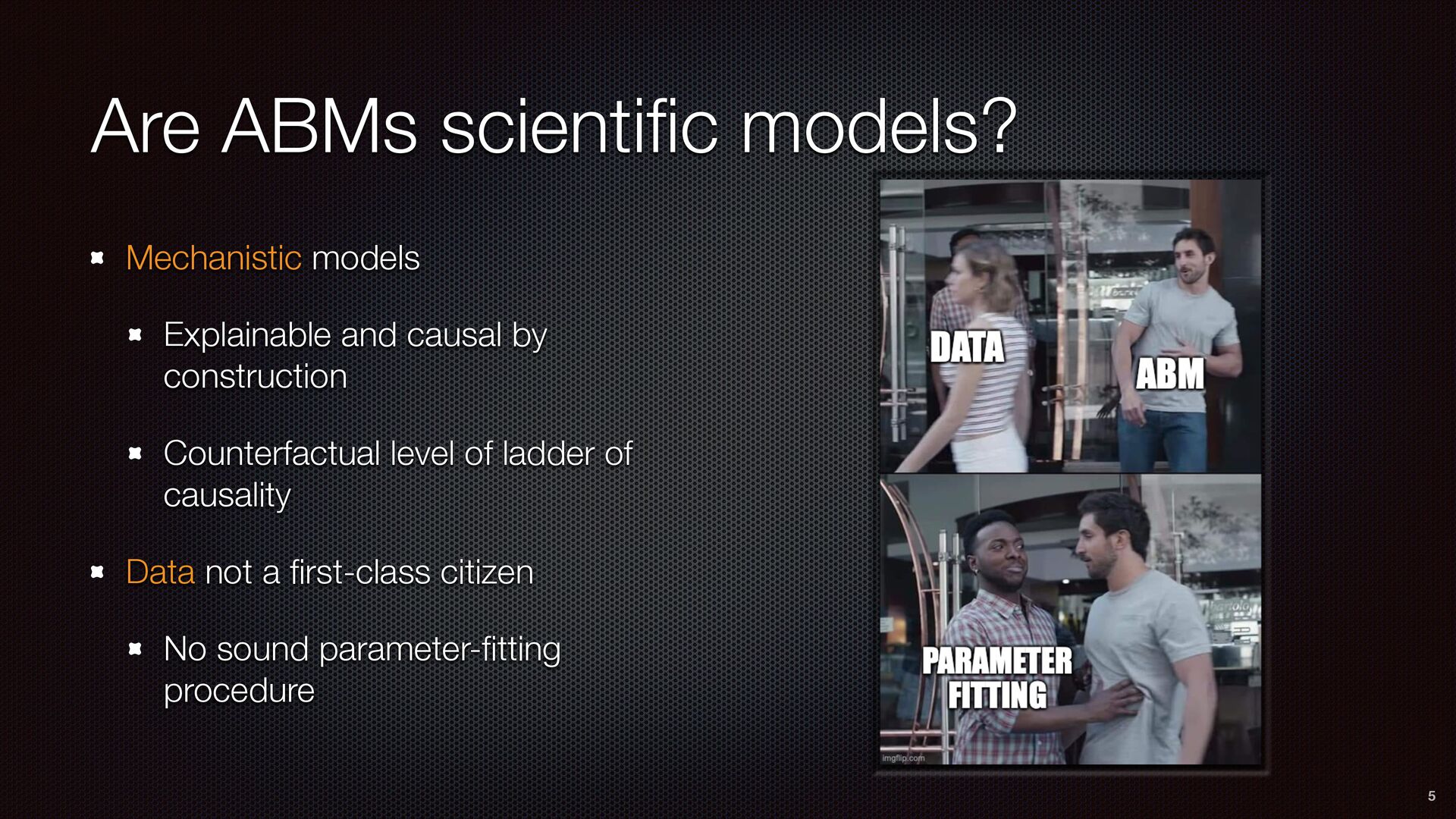
generate implications of encoded assumptions Now people use it as forecasting tool (epidemiology, economics, etc.) Calibration to set parameters from data 7
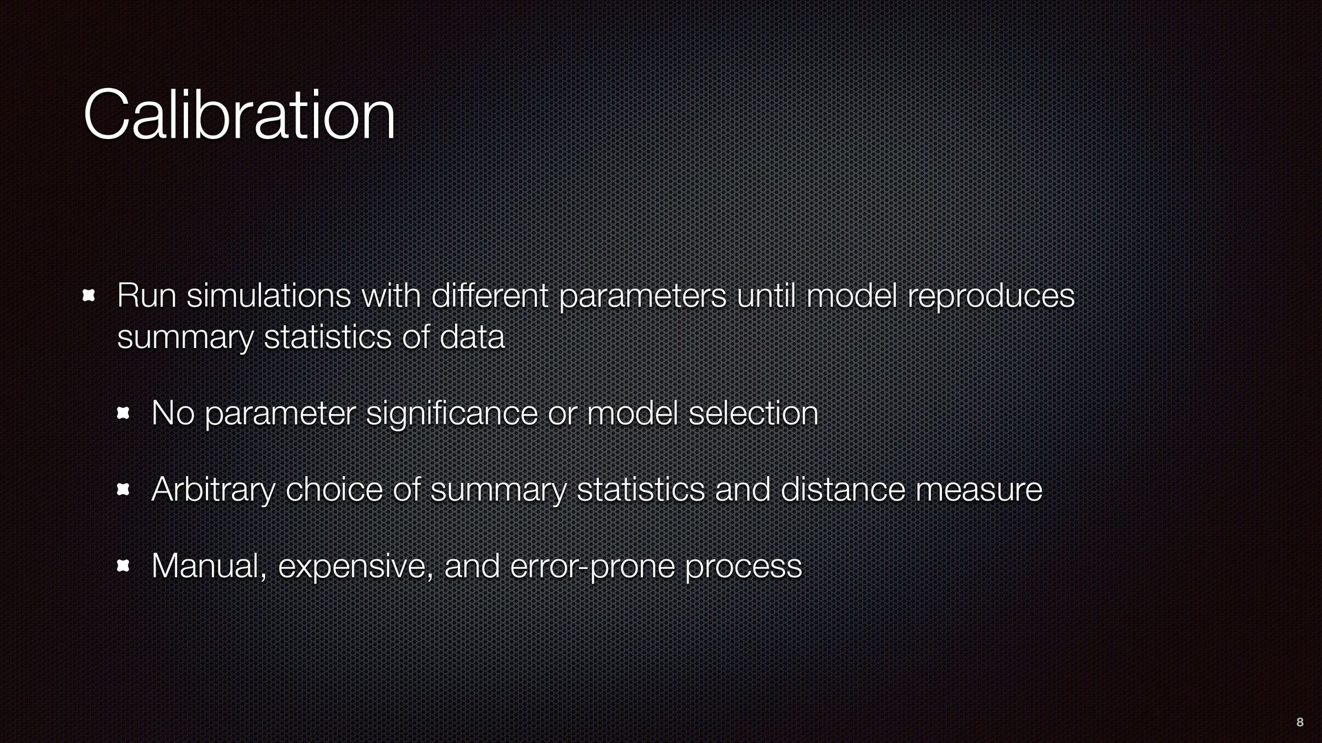
summary statistics of data No parameter signi fi cance or model selection Arbitrary choice of summary statistics and distance measure Manual, expensive, and error-prone process 8
to Daniel Bernoulli and Lagrange in the eighteenth century Fisher introduced the method as alternative to method of moments Which he criticizes for its arbitrariness in the choice of moment equations 10
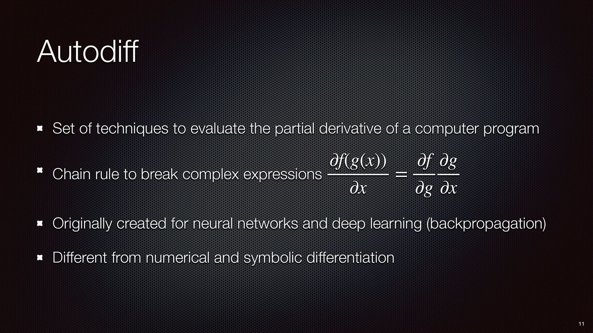
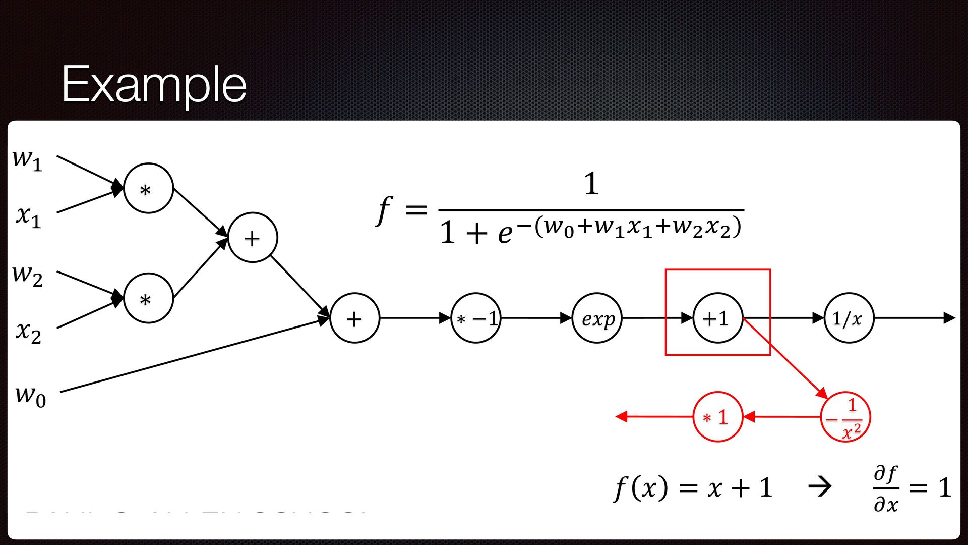
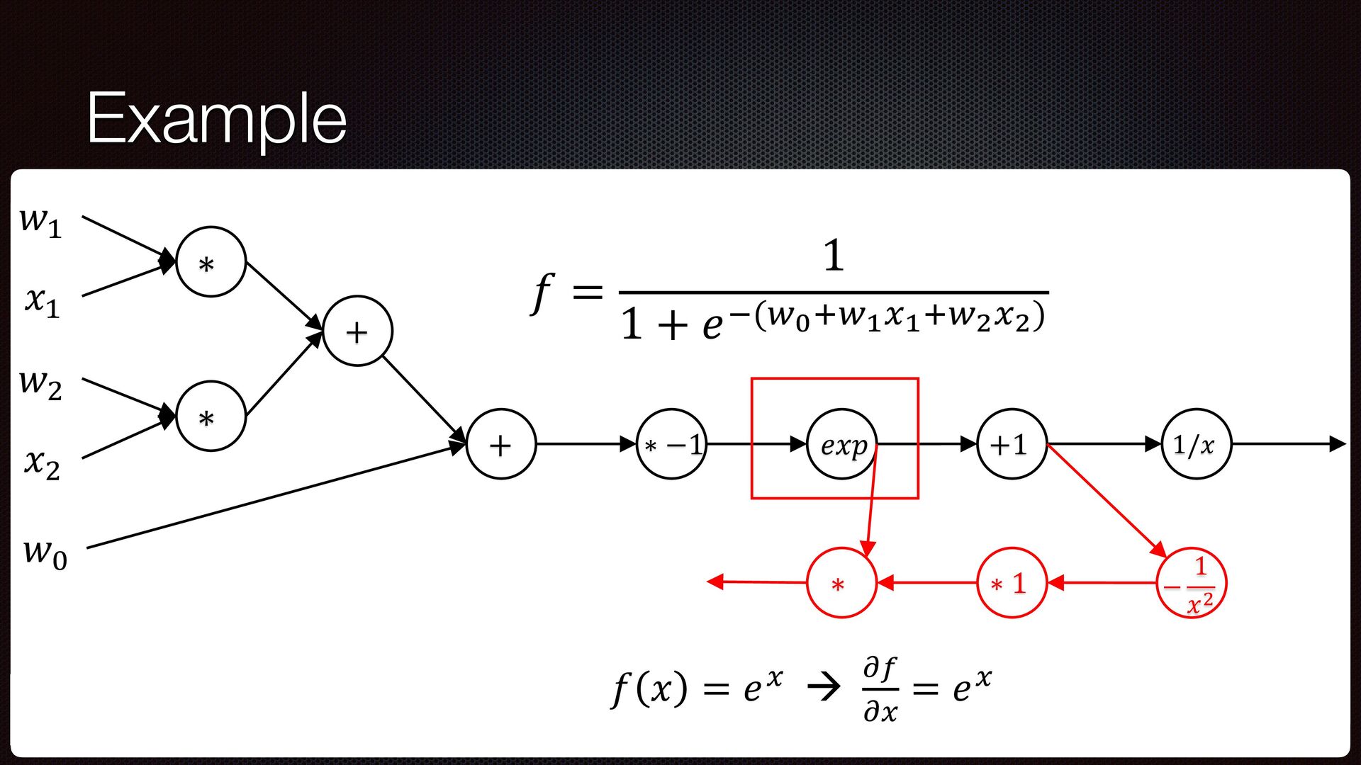
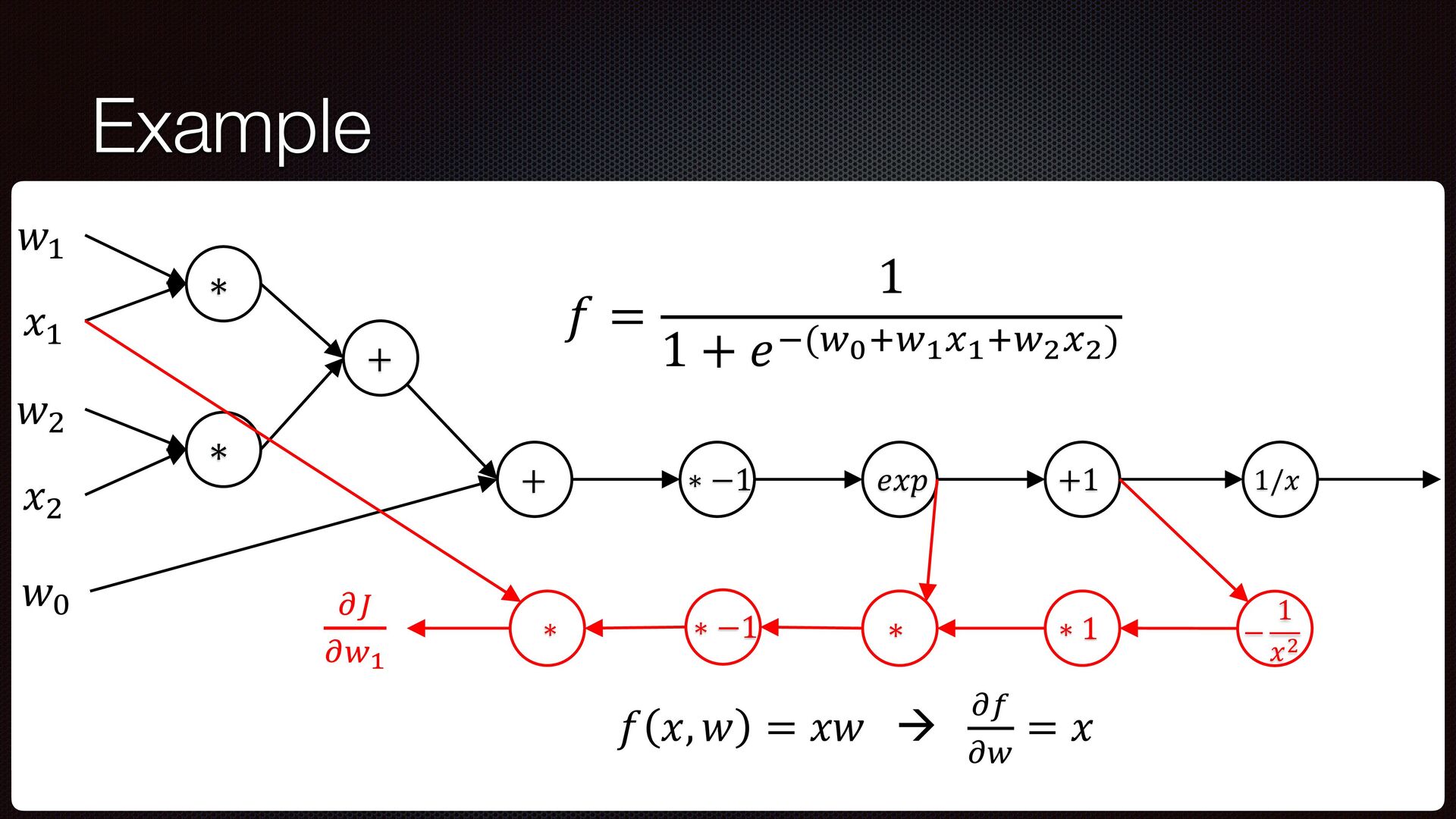
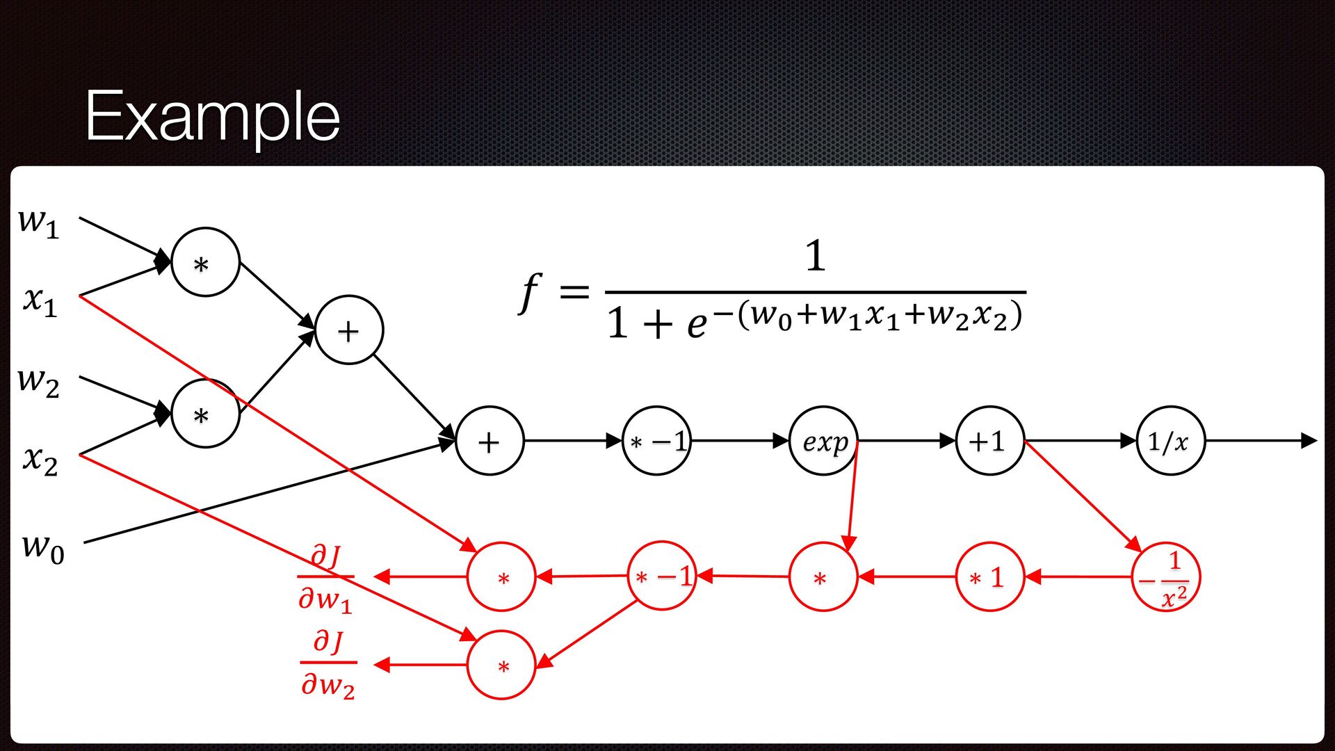
a computer program Chain rule to break complex expressions Originally created for neural networks and deep learning (backpropagation) Different from numerical and symbolic differentiation ∂f(g(x)) ∂x = ∂f ∂g ∂g ∂x 11
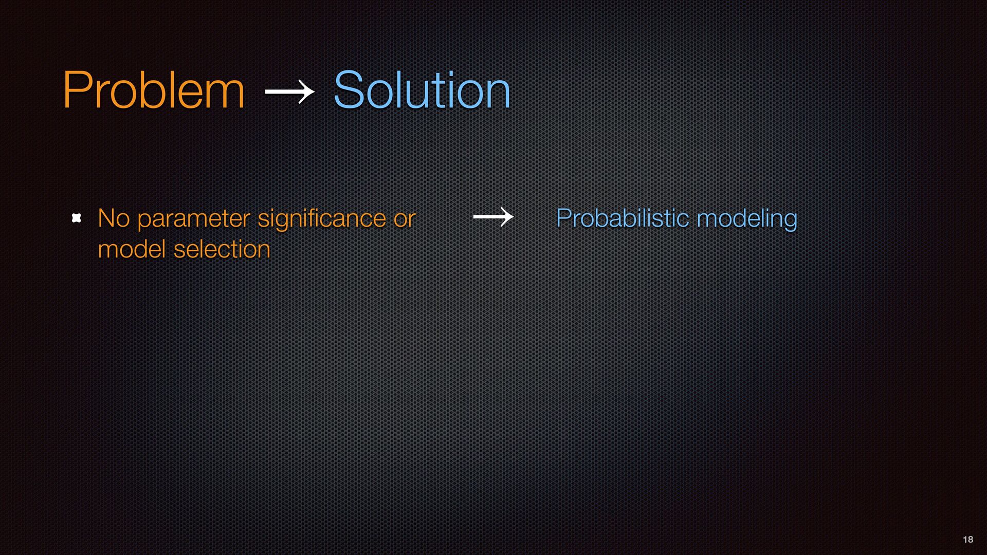
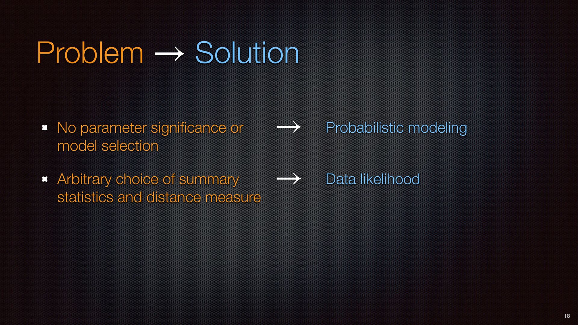
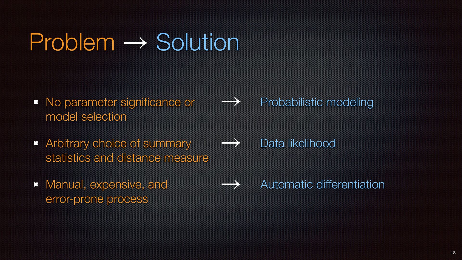
selection Arbitrary choice of summary statistics and distance measure Manual, expensive, and error-prone process Probabilistic modeling Data likelihood Automatic differentiation 18 → → →
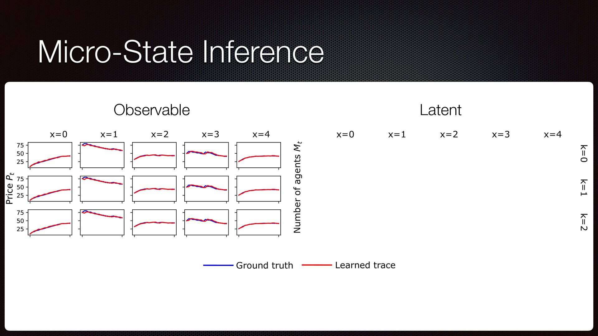
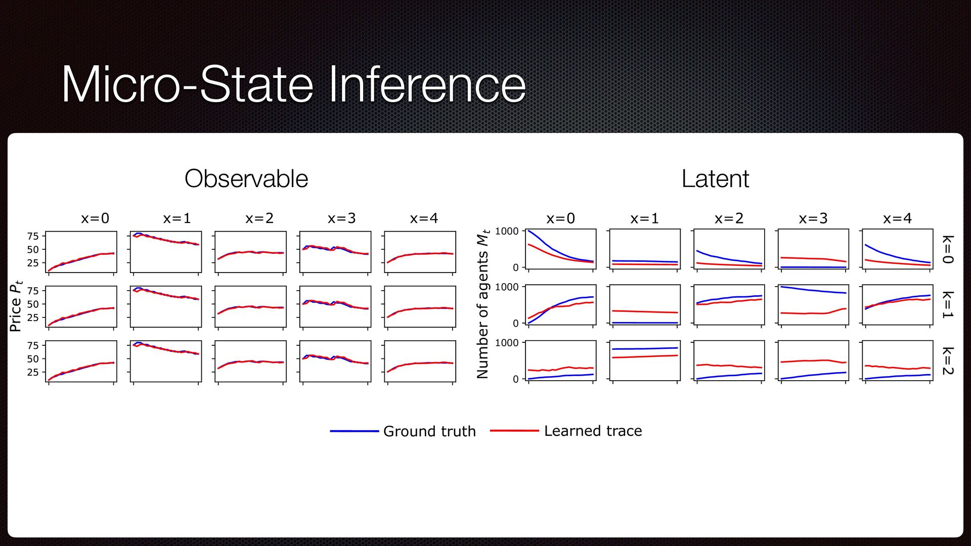
k=1 0 1000 k=2 Number of agents Mt 0 100 k=0 0 100 k=1 100 k er of buyers DB t Learned trace Ground truth Latent Observable 0 1000 x=0 x=1 x=2 x=3 k=0 x=4 0 1000 k=1 0 1000 k=2 Number of agents Mt 0 100 k=0 0 100 k=1 100 k= ber of buyers DB t Learned trace Ground truth 0 1000 x=0 x=1 x=2 x=3 k=0 x=4 1000 k=1 f agents Mt Learned trace Ground truth Micro-State Inference
k=1 0 1000 k=2 Number of agents Mt 0 100 k=0 0 100 k=1 100 k er of buyers DB t Learned trace Ground truth Latent Observable 0 1000 x=0 x=1 x=2 x=3 k=0 x=4 0 1000 k=1 0 1000 k=2 Number of agents Mt 0 100 k=0 0 100 k=1 100 k= ber of buyers DB t Learned trace Ground truth 0 1000 x=0 x=1 x=2 x=3 k=0 x=4 1000 k=1 f agents Mt Learned trace Ground truth Micro-State Inference
k=1 0 1000 k=2 Number of agents Mt 0 100 k=0 0 100 k=1 100 k er of buyers DB t Learned trace Ground truth Latent Observable 0 1000 x=0 x=1 x=2 x=3 k=0 x=4 0 1000 k=1 0 1000 k=2 Number of agents Mt 0 100 k=0 0 100 k=1 100 k= ber of buyers DB t Learned trace Ground truth 0 1000 x=0 x=1 x=2 x=3 k=0 x=4 1000 k=1 f agents Mt Learned trace Ground truth Micro-State Inference
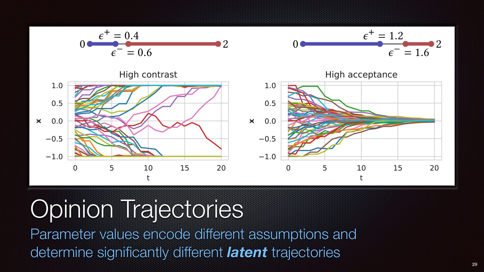
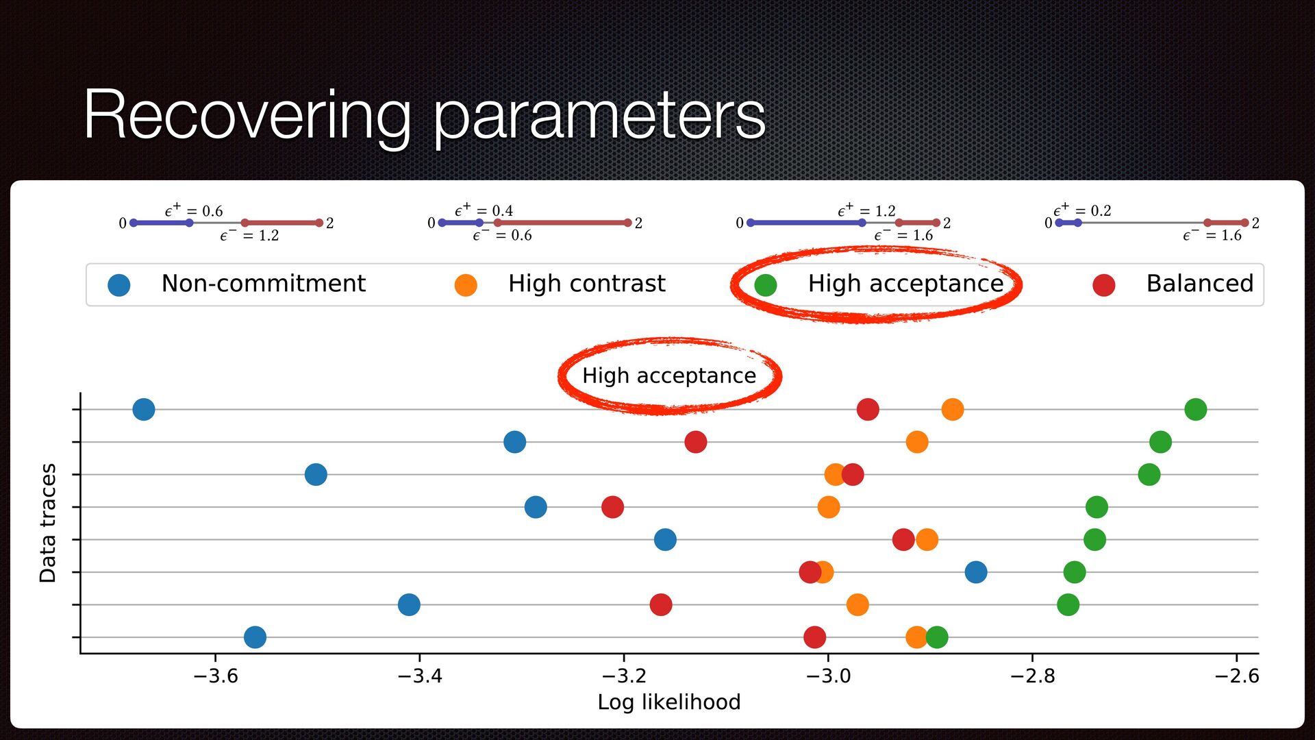
2 n+ = 1.2 n = 1.6 nthetic data traces generated in each scenario. Plots represent the opini Opinion Trajectories Parameter values encode different assumptions and determine signi fi cantly different latent trajectories 29
generated in each s 0 2 n+ = 0.6 n = 1.2 0 2 n+ = 0.4 n = 0.6 0 2 n+ = 1.2 n = 1.6 0 2 n+ = 0.2 n = 1.6 Figure 4: Examples of synthetic data traces generated in each scenario. Plots represent the opinion trajectories along time.
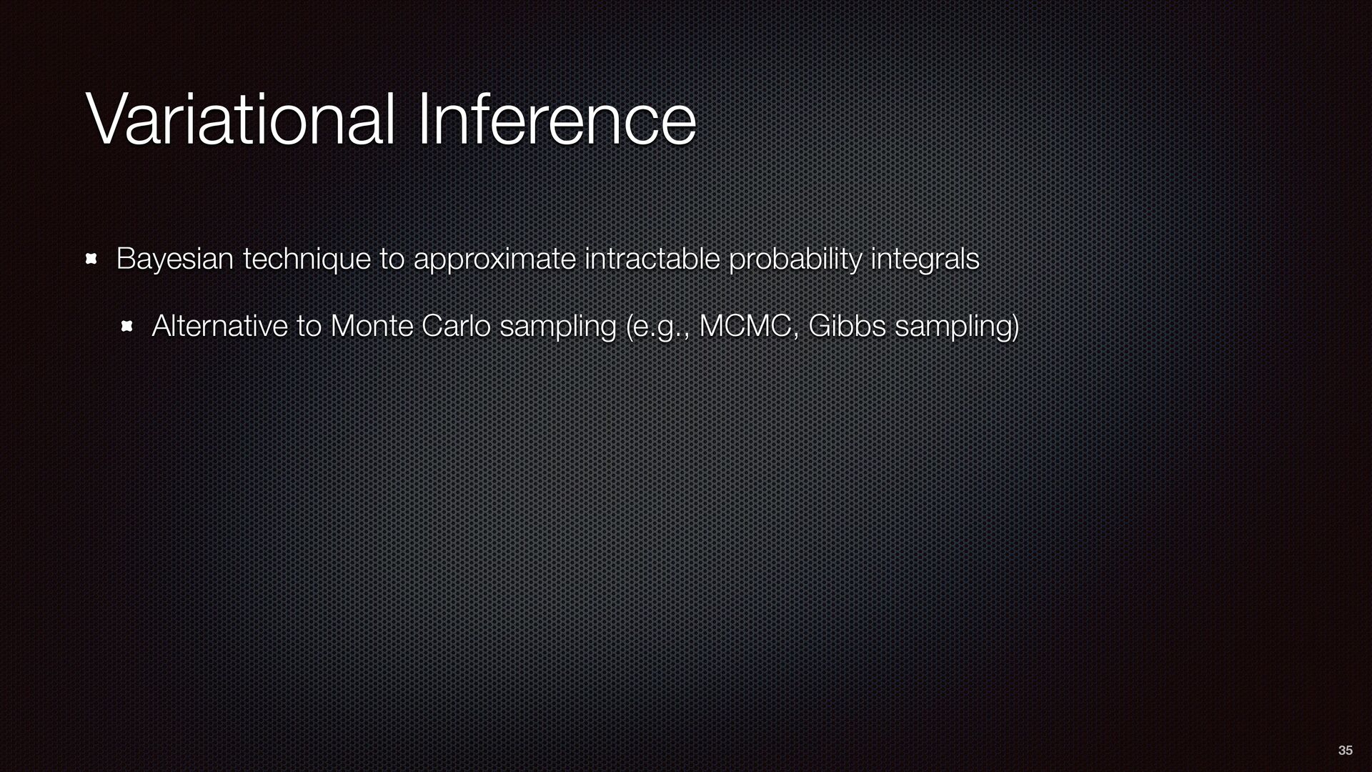
be challenging Easy to make mistakes Requires deep understanding of the data generating process Is there a way to avoid it? Variational approximation! 34
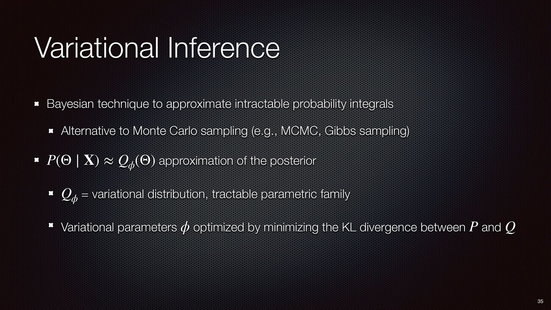
to Monte Carlo sampling (e.g., MCMC, Gibbs sampling) approximation of the posterior = variational distribution, tractable parametric family Variational parameters optimized by minimizing the KL divergence between and P(Θ ∣ X) ≈ Qϕ (Θ) Qϕ ϕ P Q 35
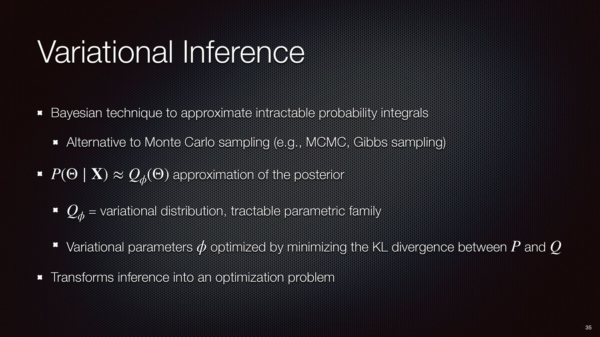
to Monte Carlo sampling (e.g., MCMC, Gibbs sampling) approximation of the posterior = variational distribution, tractable parametric family Variational parameters optimized by minimizing the KL divergence between and P(Θ ∣ X) ≈ Qϕ (Θ) Qϕ ϕ P Q Transforms inference into an optimization problem 35
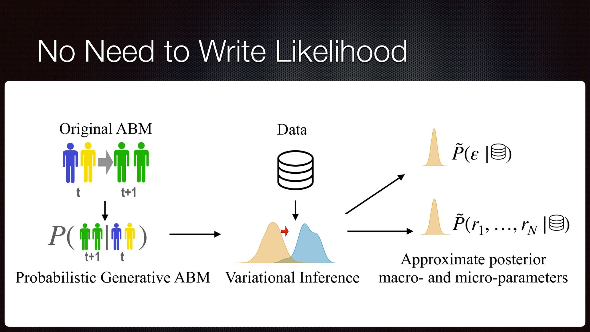
ABM Probabilistic Generative ABM Variational Inference Data Approximate posterior macro- and micro-parameters ˜ P(ε ∣ ) ˜ P(r 1 , …, r N ∣ ) t t+1 t+1 t
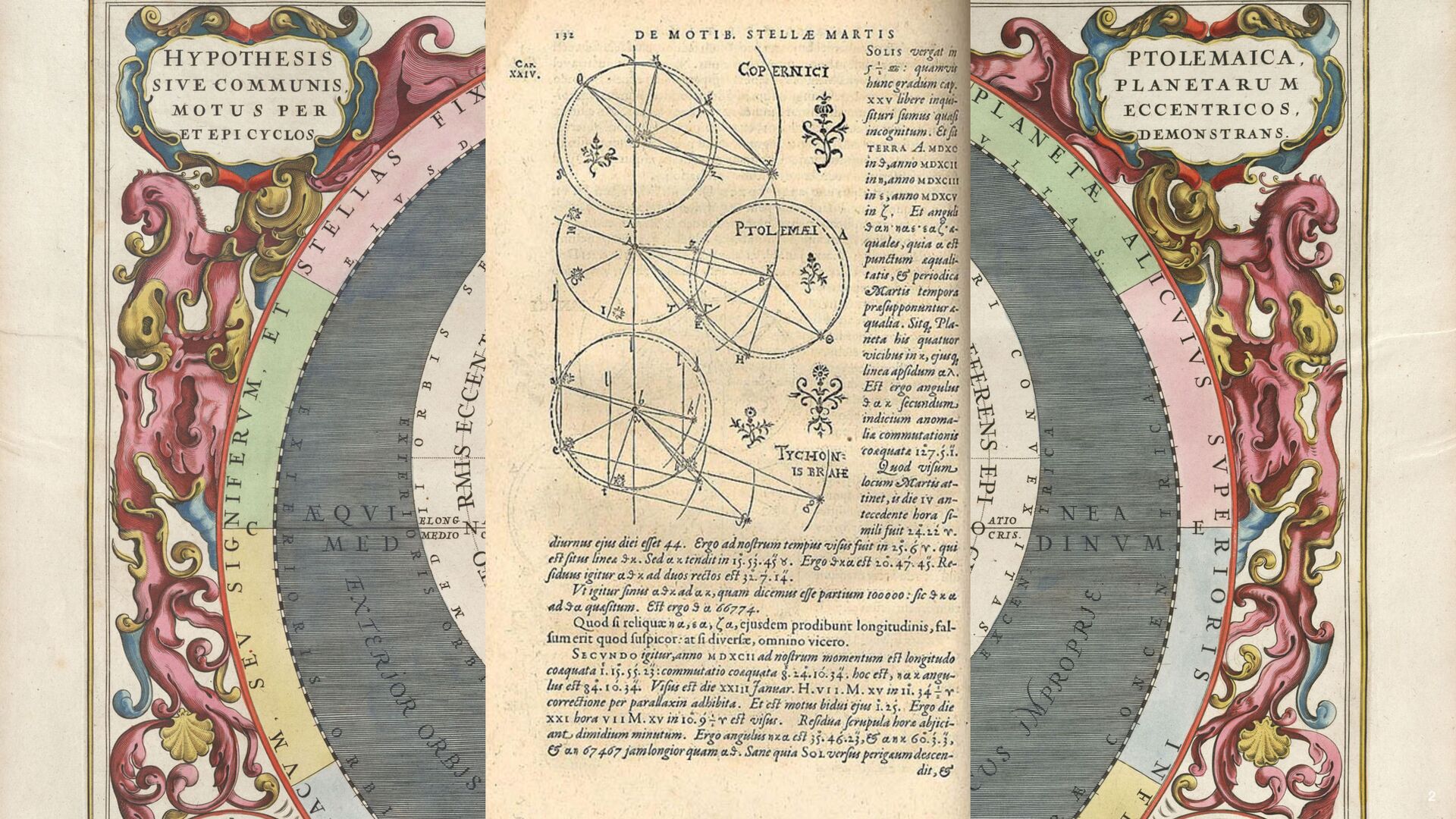
for the data-generating process Learn latent variables of models Forecasting and predictions Model selection Use data to fi gure out which models work (Ptolemy vs Kepler) Bring ABM in line with statistical models (and scienti fi c ones) 41
Opinion Dynamics From Social Traces” KDD 2020 C. Monti, M. Pangallo, G. De Francisci Morales, F. Bonchi “On Learning Agent-Based Models from Data” Scienti fi c Reports 2023 J. Lenti, C. Monti, G. De Francisci Morales “Likelihood-Based Methods Improve Parameter Estimation in Opinion Dynamics Models” WSDM 2024 J. Lenti, F. Silvestri, G. De Francisci Morales “Variational Inference of Parameters in Opinion Dynamics Models” arXiv:2403.05358 2024 42 [email protected] https://gdfm.me @gdfm7