Machine Learning Lectures - Decision Trees

Transcript

1. Machine Learning Lectures Decision Trees Gregory Ditzler gregory.ditzler@gmail.com February 24, 2024 1 / 33
2. Overview 1. Motivation 2. Decision Trees 3. Examples 2 / 33
3. Motivation 3 / 33
4. Motivation • Decision trees are a fundamentally different approach to building a machine learning model than we have studied in the past. • Most of the approaches we learned about are a “black” box from the perspective of the user. That is if a model predicts y, why did the model choose y? SVM: y(x) = j∈SV αj yj k(xj , x) + b • Trees are not based on a measure of distance, rather they are a part of a more general class of approaches known as graphical models • Trees can handle nominal (categorical), as well as ordinal and cardinal (numeric) data, while most other classifiers require such data to be transformed to ordinal data. • Given a decision, trees can be used to explain exactly how we reach as decision. 4 / 33
5. Decision Trees 5 / 33
6. Decision Trees Tree-based Models • Classification and regression trees, or CART (Breiman et al., 1984), and C4.5 (Quinlan, 1986) are two of the more popular methods for generating decision trees. • Decision trees provide a natural setting to handle data for containing categorical variables, but can still use continuous variables. Pros & Cons • Decision trees are unstable classifiers – a small change on the input can produce a large change on the output. con • Prone to overfitting. con • Easy to interpret! pro 6 / 33
7. Components to a Tree • The root node represents the first question (rule) to be answered by the tree. Usually, the root is associated with the most important attribute (feature). • The root node is connected to other internal nodes called descendents, with directional links, called branches, that represent the values of the attributes for the node. Each descendent node is connected to one parent node. Each decision made at a node splits the data through the branches. The part of the tree that follows a node is called a subtree. • A node that does not have any descendents is called a leaf node (or terminal node). Each leaf node is associated with one of the category labels, i.e., classes. 7 / 33
8. Visualizing a Tree x2 ≥ δ10 ω1 x1 ≥ δ20 x5 ≥ δ30 ω1 ω2 ω1 Given a dataset D := {(xi, yi)}n i=1 , how do we construct a decision tree and learn the thresholds δ10, δ20 and δ30? 8 / 33
9. A binary-split decision tree and feature space partition A B C D E θ1 θ4 θ2 θ3 x1 x2 x1 > θ1 x2 > θ3 x1 θ4 x2 θ2 A B C D E Illustration of the feature space partitioning of x = [x1, x2]T into five regions (left). The binary-tree used to partition the feature space is done using the binary tree on the right. 9 / 33
10. What do we need to think about if we learn a tree? 1. How many decision outcomes, B, (or splits) will there be at each node? If B = 2, we have a binary tree, where each question has a yes or no answer. Any multi- valued tree can be converted into a binary tree. 2. Which property (attribute) be tested at each node? 3. When should a node be declared a leaf node? When should tree construction end? 4. Should the tree be pruned (to prevent over-fitting), and if so, how? 5. If a leaf node is impure, what category label should be assigned? 6. How should missing data be handled? 10 / 33
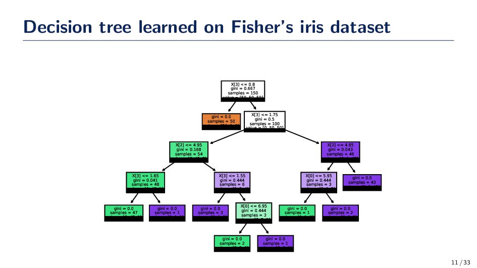
11. Decision tree learned on Fisher’s iris dataset gini = 0.0 samples = 2 value = [0, 2, 0] gini = 0.0 samples = 1 value = [0, 0, 1] gini = 0.0 samples = 47 value = [0, 47, 0] gini = 0.0 samples = 1 value = [0, 0, 1] gini = 0.0 samples = 3 value = [0, 0, 3] X[0] <= 6.95 gini = 0.444 samples = 3 value = [0, 2, 1] gini = 0.0 samples = 1 value = [0, 1, 0] gini = 0.0 samples = 2 value = [0, 0, 2] X[3] <= 1.65 gini = 0.041 samples = 48 value = [0, 47, 1] X[3] <= 1.55 gini = 0.444 samples = 6 value = [0, 2, 4] X[0] <= 5.95 gini = 0.444 samples = 3 value = [0, 1, 2] gini = 0.0 samples = 43 value = [0, 0, 43] X[2] <= 4.95 gini = 0.168 samples = 54 value = [0, 49, 5] X[2] <= 4.85 gini = 0.043 samples = 46 value = [0, 1, 45] gini = 0.0 samples = 50 value = [50, 0, 0] X[3] <= 1.75 gini = 0.5 samples = 100 value = [0, 50, 50] X[3] <= 0.8 gini = 0.667 samples = 150 value = [50, 50, 50] 11 / 33
12. Decision Trees • Decision trees are models that represent a hierarchy of how we arrived at a decision. • These trees allow us to re-trace our steps back through the tree to see exactly how we arrived at any particular decision. Definition • A dataset D := {(xi, yi)}n i=1 is available at the time of training. For the moment, we are going to assume that yi ∈ Y. • Let the ci be the ith class of the dataset, and m indicate an arbitrary node in the tree. There are Nm samples that arrive at the mth node and Ni m be the number of samples from class ci at the mth node. Nm = K i=1 Ni m , fm(x) : xℓ > wm,0 where fm(x) is the decision function that thresholds the ℓth feature. 12 / 33
13. Setting Up the Problem How are we going to split at a node? • Given that a data sample reaches the mth node, the probability that it belongs to class ci is given by: P(ci|x, m) = pi m = Ni m Nm If a node is pure then pi m is either 0 or 1. In this situation, there is no need to split. • pi m = 0 if all points at node m are NOT ci • pi m = 1 if all points at node m are ci • In general, there will be a spectrum on the interval [0, 1] • We need a way to capture the uncertainty at a node so we can look for the split that leads to the largest reduction in uncertainty at the next nodes. 13 / 33
14. Capturing Uncertainty Entropy of a Random Variable One way to capture uncertainty is entropy. More formally, Hm = − K i=1 pi m log2 (pi m ) • The figure on the right shows the entropy of a Bernoulli random variable. • The uncertainty – or entropy – is the largest when p = 1/2. 0.0 0.2 0.4 0.6 0.8 1.0 p 0.0 0.2 0.4 0.6 0.8 1.0 Entropy (Bits) Note we can compute Hm then choose and split action j that will give another value for entropy. 14 / 33
15. Choose the Split that Maximally Reduces Entropy Let j be the outcome for performing a split (e.g., we chose a feature and threshold). Given that we are at node m, the test (i.e., x > wm,0) gives the probability P(ci|x, m, j) = pi m,j = Ni m,j Nm,j and the total impurity becomes H′ m = − n j=1 Nm,j Nm K i=1 pi m,j log2 (pi m,j ) The function fm(x) can be used to split the tree, and ideally it is the split that reduces entropy the most (e.g., max(Hm − H′ m )). So how do we find wm,0. 15 / 33
16. How are we going to find wm,0 ? • At first glance, finding wm,0 might seem like a daunting task; however, this is not the case! This is a 1D optimization task. • For any arbitrary feature, we do not need to consider all possible splits. We only need to consider the splits were the data (on a 1D line) have a neighbor that is from a different class. 4 3 2 1 0 1 2 3 Feature Value Class 1 Class 2 We do not need to consider multiple thresholds between [−4, −3] since these splits do not impact the change in entropy. 16 / 33
17. Other ways to measure impurity: Gini’s Index Definition Let p(i) be the probability of picking a data point with class i. Then the Gini index is given by: G = K i=1 p(i)(1 − p(i)) A Gini Impurity of 0 is the lowest and best possible impurity. It can only be achieved when everything is the same class. We choose the split that leads to the smallest impurity. • Goal: Measure the Gini impurity after the split then look at the difference between impurity before and after the split. 17 / 33
18. Gini Impurity Example 0.0 0.5 1.0 1.5 2.0 2.5 3.0 x1 0.0 0.5 1.0 1.5 2.0 2.5 3.0 x2 Class0 Class1 Begin by calculating the impurity of the left & right spaces, then weight the impurity by the ratio of samples. Gleft = 0 Gright = 1 6 1 − 1 6 + 5 6 1 − 5 6 = 5 18 ≈ 0.278 Gtot = 4 10 · 0 + 6 10 · 0.278 = 0.167 Assume that the impurity from the previous split was 1/2. Thus, the amount of impurity removed with this split is: 0.5 − 0.167 = 0.333. This is the Gini gain (larger is better). 18 / 33
19. DecisionTreeClassifier with Gini Impurity from sklearn.datasets import load_iris from sklearn.model_selection import cross_val_score from sklearn.tree import DecisionTreeClassifier # criterion = ’entropy’, ’log_loss’, ’gini’ clf = DecisionTreeClassifier(criterion=’gini’) iris = load_iris() cross_val_score(clf, iris.data, iris.target, cv=10) https://scikit-learn.org/stable/modules/tree.html# tree-mathematical-formulation 19 / 33
20. Stopping Criteria • Decision trees are extremely prone to overfit to a training dataset. In fact, any decision tree can perfectly fit the training data! • This can easily be explained by looking at a tree that is grown until there is exactly one training sample in the dataset at a leaf node. • How can we prevent the tree from overfitting? We’re going to need to think of a few criteria to decide when to stop growing the tree. • There are many ways we can implement early stopping with a decision tree and there are several that are typically implemented at the same time. 20 / 33
21. Stopping Criteria Minimum Sample Splitting Criteria A “current” leaf node during training must have more than Nsplit samples at the leaf to consider a split. If there are less than Nsplit samples then splits below the node are not considered in the future. Maximum Tree Depth Do not grow the tree past a pre-specified depth. Minimum Leaf Sample Criteria A split point at any depth will only be considered if it leaves at least the number of training samples in each of the left and right branches. This may have the effect of smoothing the model. 21 / 33
22. Stopping Criteria Hypothesis Testing We can use a hypothesis test to determine whether the split is beneficial or not. Pruning A tree is fully grown until all leaves have minimum impurity. All pairs of neighboring leaf nodes (those with the same parent node) are considered for elimination. For example, we could grow the tree and perform error-based pruning to shrink the tree such that it still has an acceptable error. 22 / 33
23. The Horizon Effect The Horizon Effect • Occasionally, stopped splitting suffers from the lack of sufficient look ahead, a phenomenon known as the horizon effect. • The determination of the “optimal” split at note N is not influenced by its descendants. That is we do not look at the lower levels of the tree when we split because they are not there at the time of the split. • Growing the full tree then pruning limits the impact of the horizon effect. 23 / 33
24. Examples 24 / 33
25. Fisher Iris 4 6 8 sepal length (cm) 1 2 3 4 5 sepal width (cm) 4 6 8 sepal length (cm) 0 2 4 6 petal length (cm) 4 6 8 sepal length (cm) 0 1 2 3 petal width (cm) 2 4 sepal width (cm) 0 2 4 6 petal length (cm) 2 4 sepal width (cm) 0 1 2 3 petal width (cm) 0 5 petal length (cm) 0 1 2 3 petal width (cm) setosa versicolor virginica Decision surface of decision trees trained on pairs of features 25 / 33
26. Impact of Tree Depth: Wine Dataset 2 4 6 8 10 12 14 Max Tree Depth 0.84 0.85 0.86 0.87 0.88 0.89 Accuracy scores = [cross_val_score(tree.DecisionTreeClassifier(max_depth=d), X, y, cv=10).mean() for d in range(2,16)] 26 / 33
27. Impact of Tree Depth: Breast Cancer Dataset 2 4 6 8 10 12 14 Max Tree Depth 0.9025 0.9050 0.9075 0.9100 0.9125 0.9150 0.9175 0.9200 0.9225 Accuracy 27 / 33
28. Impurity 0.000 0.005 0.010 0.015 0.020 0.025 0.030 0.035 effective alpha 0.00 0.02 0.04 0.06 0.08 0.10 0.12 0.14 total impurity of leaves Total Impurity vs effective alpha for training set 28 / 33
29. Complexity-based pruning 0.00 0.05 0.10 0.15 0.20 0.25 0.30 alpha 0.65 0.70 0.75 0.80 0.85 0.90 0.95 1.00 accuracy Accuracy vs alpha for training and testing sets train test 29 / 33
30. Regression Trees 0 1 2 3 4 5 6 data 2.0 1.5 1.0 0.5 0.0 0.5 1.0 1.5 2.0 target training samples RegressionTree 30 / 33
31. Regression Trees Redux 0 1 2 3 4 5 6 data 2.0 1.5 1.0 0.5 0.0 0.5 1.0 1.5 2.0 target training samples RegressionTree AveragedTrees 31 / 33
32. References Christopher Bishop (2007) Pattern Recognition and Machine Learning New York, NY: Springer 1st edition. Richard Duda, Peter Hart, David Stork (2001) Pattern Classification John Wiley & Sons 2nd edition. 32 / 33
33. The End 33 / 33