Machine Learning Lectures - Linear Models

Transcript

1. Machine Learning Lectures Linear Models and Logistic Regression Gregory Ditzler gregory.ditzler@gmail.com February 24, 2024 1 / 44
2. Overview 1. Motivation 2. Linear Regression 3. Logistic Regression 4. Multi-Class Scenarios 2 / 44
3. Motivation 3 / 44
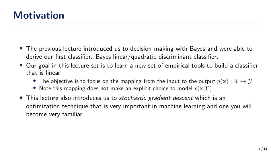
4. Motivation • The previous lecture introduced us to decision making with Bayes and were able to derive our first classifier: Bayes linear/quadratic discriminant classifier. • Our goal in this lecture set is to learn a new set of empirical tools to build a classifier that is linear • The objective is to focus on the mapping from the input to the output g(x) : X → Y • Note this mapping does not make an explicit choice to model p(x|Y ) • This lecture also introduces us to stochastic gradient descent which is an optimization technique that is very important in machine learning and one you will become very familiar. 4 / 44
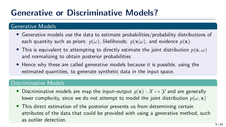
5. Generative or Discriminative Models? Generative Models • Generative models use the data to estimate probabilities/probability distributions of each quantity such as priors: p(ω), likelihoods: p(x|ω), and evidence p(x). • This is equivalent to attempting to directly estimate the joint distribution p(x, ω) and normalizing to obtain posterior probabilities • Hence why these are called generative models because it is possible, using the estimated quantities, to generate synthetic data in the input space. Discriminative Models • Discriminative models are map the input–output g(x) : X → Y and are generally lower complexity, since we do not attempt to model the joint distribution p(ω, x) • This direct estimation of the posterior prevents us from determining certain attributes of the data that could be provided with using a generative method, such as outlier detection. 5 / 44
6. Linear Regression 6 / 44
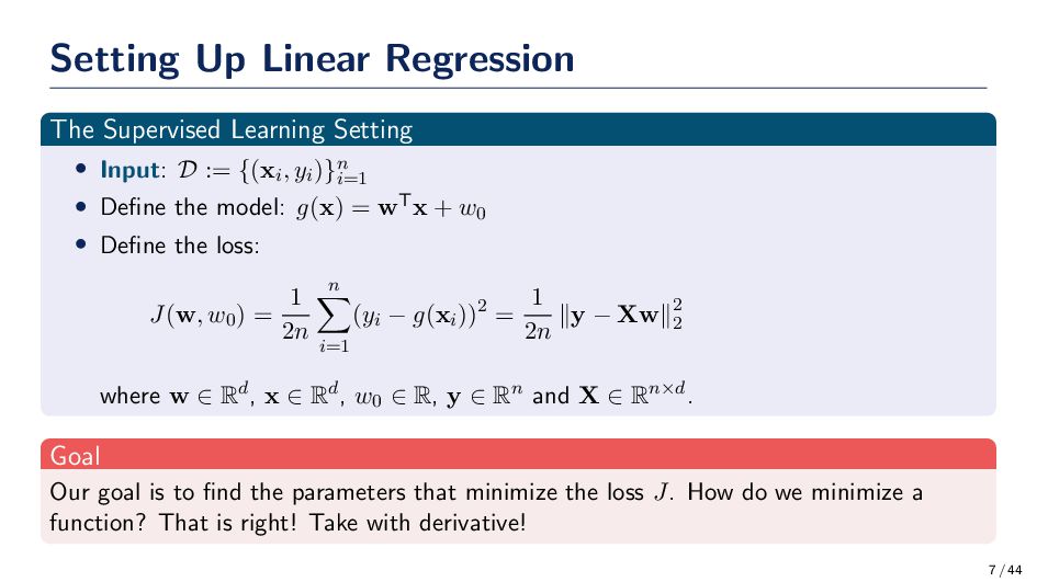
7. Setting Up Linear Regression The Supervised Learning Setting • Input: D := {(xi, yi)}n i=1 • Define the model: g(x) = wTx + w0 • Define the loss: J(w, w0) = 1 2n n i=1 (yi − g(xi))2 = 1 2n ∥y − Xw∥2 2 where w ∈ Rd, x ∈ Rd, w0 ∈ R, y ∈ Rn and X ∈ Rn×d. Goal Our goal is to find the parameters that minimize the loss J. How do we minimize a function? That is right! Take with derivative! 7 / 44
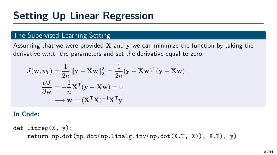
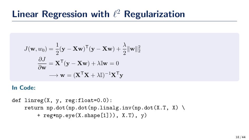
8. Setting Up Linear Regression The Supervised Learning Setting Assuming that we were provided X and y we can minimize the function by taking the derivative w.r.t. the parameters and set the derivative equal to zero. J(w, w0) = 1 2n ∥y − Xw∥2 2 = 1 2n (y − Xw)T(y − Xw) ∂J ∂w = − 1 n XT(y − Xw) = 0 −→ w = (XTX)−1XTy In Code: def linreg(X, y): return np.dot(np.dot(np.linalg.inv(np.dot(X.T, X)), X.T), y) 8 / 44
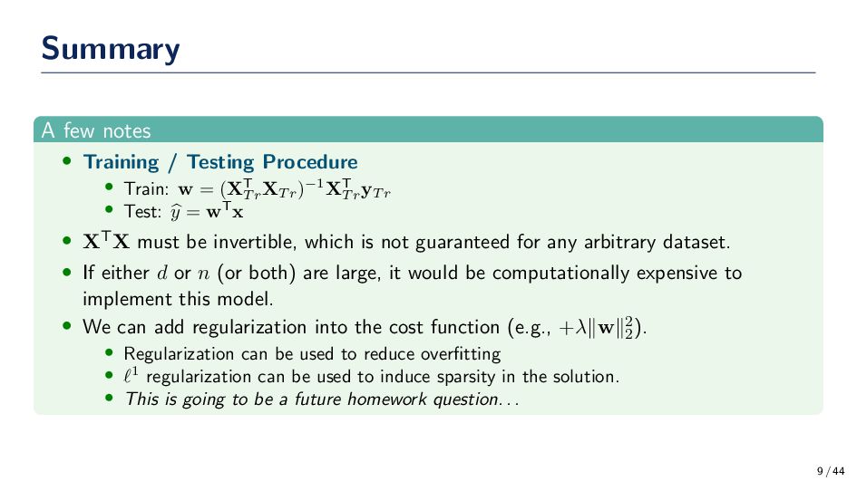
9. Summary A few notes • Training / Testing Procedure • Train: w = (XT T r XT r )−1XT T r yT r • Test: y = wTx • XTX must be invertible, which is not guaranteed for any arbitrary dataset. • If either d or n (or both) are large, it would be computationally expensive to implement this model. • We can add regularization into the cost function (e.g., +λ∥w∥2 2 ). • Regularization can be used to reduce overfitting • ℓ1 regularization can be used to induce sparsity in the solution. • This is going to be a future homework question. . . 9 / 44
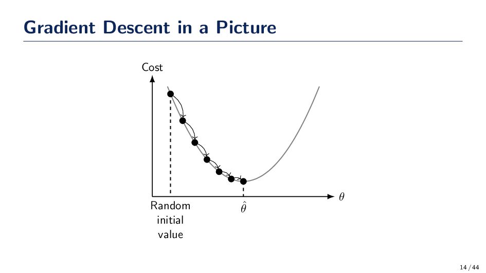
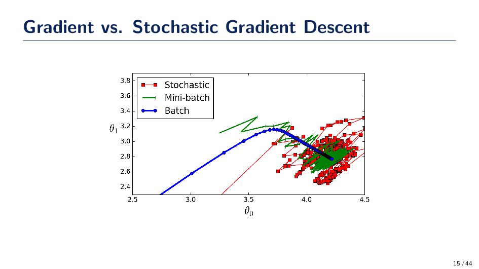
10. Motivating (Stochastic) Gradient Descent • Linear regression provided us with a closed-form solution to find the parameters w; however, we can see there are situations where using the closed-form expression is not going to be feasible. • Gradient Descent is a first-order iterative optimization algorithm for finding a local minimum of a differentiable function. In the closed-form scenario, we take one step! • With stochastic gradient descent, we can average the gradients of a few data to take a small step in the direction of the parameters that reduces the cost function. 10 / 44
11. Gradient Descent 4 2 0 2 4 x 2 4 6 8 10 f(x) Direction of the gradient Direction of the gradient descent w(τ + 1) = w(τ) + ∆w(τ) 11 / 44
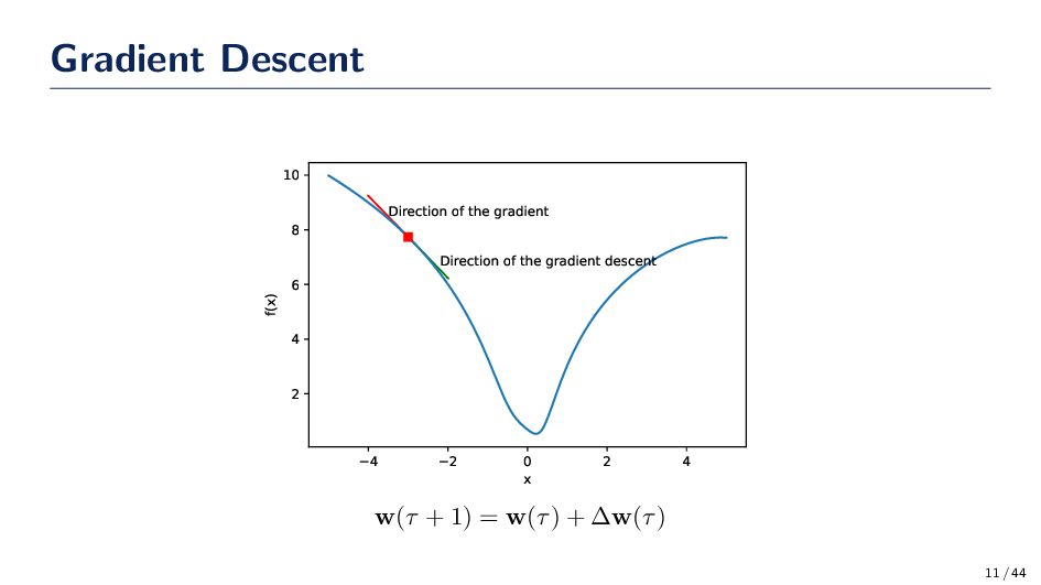
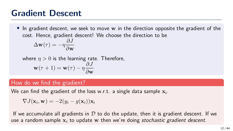
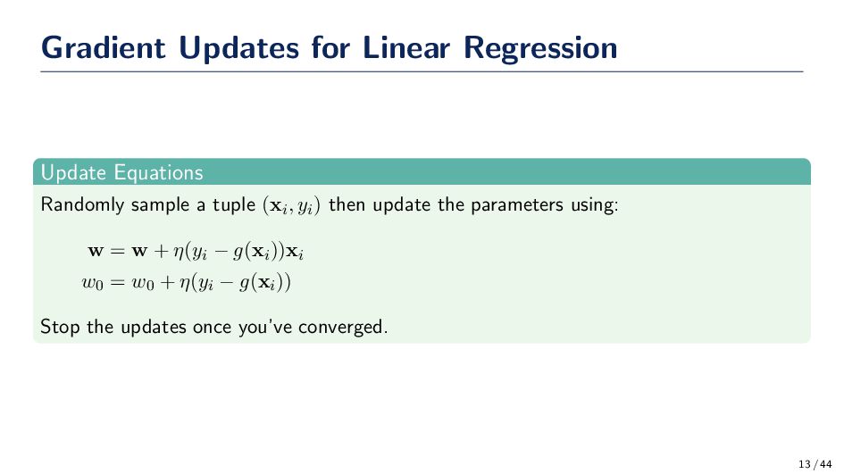
12. Gradient Descent • In gradient descent, we seek to move w in the direction opposite the gradient of the cost. Hence, gradient descent! We choose the direction to be ∆w(τ) = −η ∂J ∂w where η > 0 is the learning rate. Therefore, w(τ + 1) = w(τ) − η ∂J ∂w How do we find the gradient? We can find the gradient of the loss w.r.t. a single data sample xi. ∇J(xi, w) = −2(yi − g(xi))xi If we accumulate all gradients in D to do the update, then it is gradient descent. If we use a random sample xi to update w then we’re doing stochastic gradient descent. 12 / 44
13. Gradient Updates for Linear Regression Update Equations Randomly sample a tuple (xi, yi) then update the parameters using: w = w + η(yi − g(xi))xi w0 = w0 + η(yi − g(xi)) Stop the updates once you’ve converged. 13 / 44
14. Gradient Descent in a Picture θ Cost Random initial value ˆ θ 14 / 44
15. Gradient vs. Stochastic Gradient Descent 15 / 44
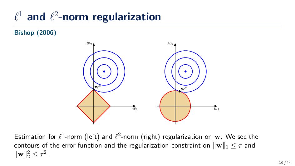
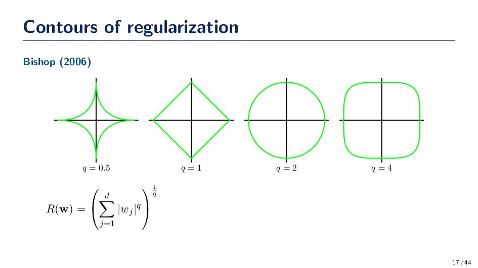
16. ℓ1 and ℓ2-norm regularization Bishop (2006) w1 w2 w w1 w2 w Estimation for ℓ1-norm (left) and ℓ2-norm (right) regularization on w. We see the contours of the error function and the regularization constraint on ∥w∥1 ≤ τ and ∥w∥2 2 ≤ τ2. 16 / 44
17. Contours of regularization Bishop (2006) q = 0.5 q = 1 q = 2 q = 4 R(w) =   d j=1 |wj|q   1 q 17 / 44
18. Linear Regression with ℓ2 Regularization J(w, w0) = 1 2 (y − Xw)T(y − Xw) + λ 2 ∥w∥2 2 ∂J ∂w = XT(y − Xw) + λIw = 0 −→ w = (XTX + λI)−1XTy In Code: def linreg(X, y, reg:float=0.0): return np.dot(np.dot(np.linalg.inv(np.dot(X.T, X) \ + reg*np.eye(X.shape[1])), X.T), y) 18 / 44
19. Regularized Linear Models: g(x) = wTx + w0 Ridge Regression (Tikhonov regularization) JRR = 1 2n n i=1 (yi − g(xi))2 + λ 2 d j=1 w2 j LASSO JL = 1 2n n i=1 (yi − g(xi))2 + λ d j=1 |wj| Elastic Nets: α ∈ [0, 1] JEN = 1 2n n i=1 (yi − g(xi))2 + (1 − α) λ2 2 d j=1 w2 j + αλ1 d j=1 |wj| 19 / 44
20. Lasso & Elastic Net Examples 1.5 1.0 0.5 0.0 0.5 -Log(alpha) 10 5 0 5 10 15 20 25 coefficients Lasso and Elastic-Net Paths Lasso Elastic-Net 1.5 1.0 0.5 0.0 0.5 -Log(alpha) 10 5 0 5 10 15 20 25 coefficients Lasso and positive Lasso Lasso positive Lasso 1.5 1.0 0.5 0.0 0.5 -Log(alpha) 10 5 0 5 10 15 20 25 coefficients Elastic-Net and positive Elastic-Net Elastic-Net positive Elastic-Net 20 / 44
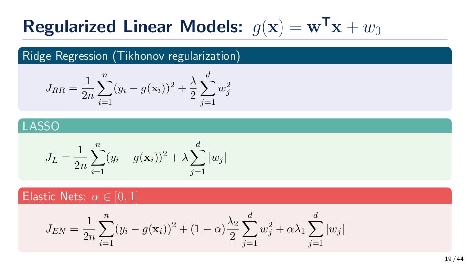
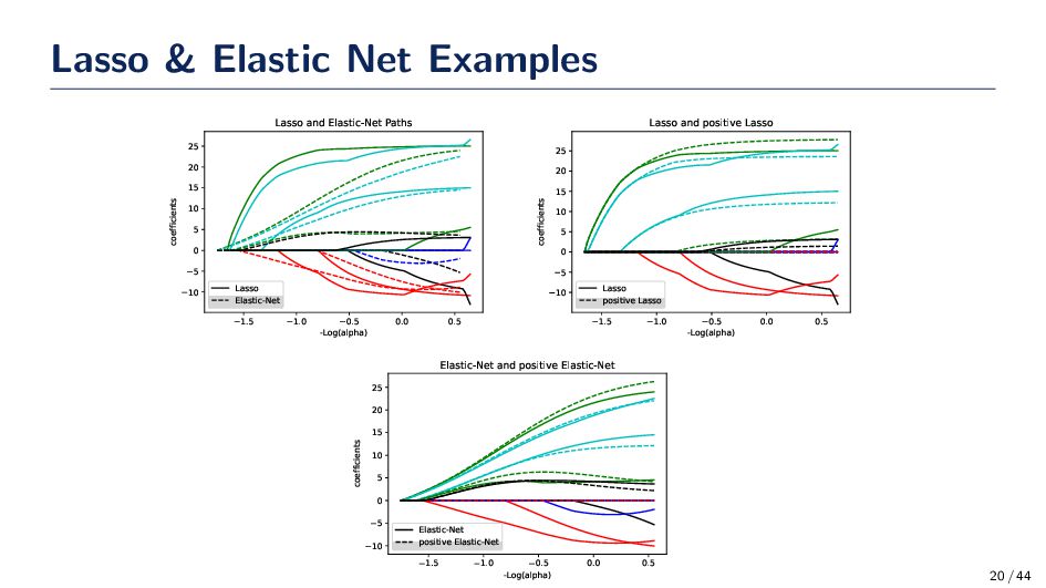
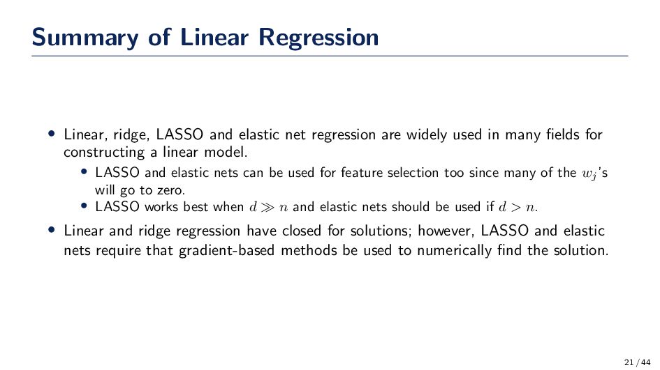
21. Summary of Linear Regression • Linear, ridge, LASSO and elastic net regression are widely used in many fields for constructing a linear model. • LASSO and elastic nets can be used for feature selection too since many of the wj ’s will go to zero. • LASSO works best when d ≫ n and elastic nets should be used if d > n. • Linear and ridge regression have closed for solutions; however, LASSO and elastic nets require that gradient-based methods be used to numerically find the solution. 21 / 44
22. Logistic Regression 22 / 44
23. Motivating Logistic Regression • Linear regression provides us a measure of how close a sample is to the decision boundary from the function g(x). That is the larger |g(x)| the farther a sample is from the plane. • Unfortunately, this score does not directly correspond to the probability that a sample belongs to a class. • We could try to think of a heuristic to connect g(x) to a probability; however, let us try to derive a relationship. • We’re going to need to go back to the lecture on Bayes to get the conversation of logistic regression started. • Linear regression ended up having a very convenient solution (i.e., it was a convex optimization task) and we want to try to obtain a similar results – if possible. • Goal: Start with Bayes theorem to find a linear predictive model that can provide an estimate of the posterior probability. 23 / 44
24. Motivating Logistic Regression P(Y = 1|x) = P(Y = 1)P(x|Y = 1) P(x) = P(Y = 1)P(x|Y = 1) P(Y = 1)P(x|Y = 1) + P(Y = 0)P(x|Y = 0) = 1 1 + P(Y =0)P(x|Y =0) P(Y =1)P(x|Y =1) = 1 1 + exp log P(Y =0)P(x|Y =0) P(Y =1)P(x|Y =1) = 1 1 + exp − log P(Y =1)P(x|Y =1) P(Y =0)P(x|Y =0) = 1 1 + exp − log P(Y =1) P(Y =0) + d j=1 log P(xj|Y =1) P(xj|Y =0) 24 / 44
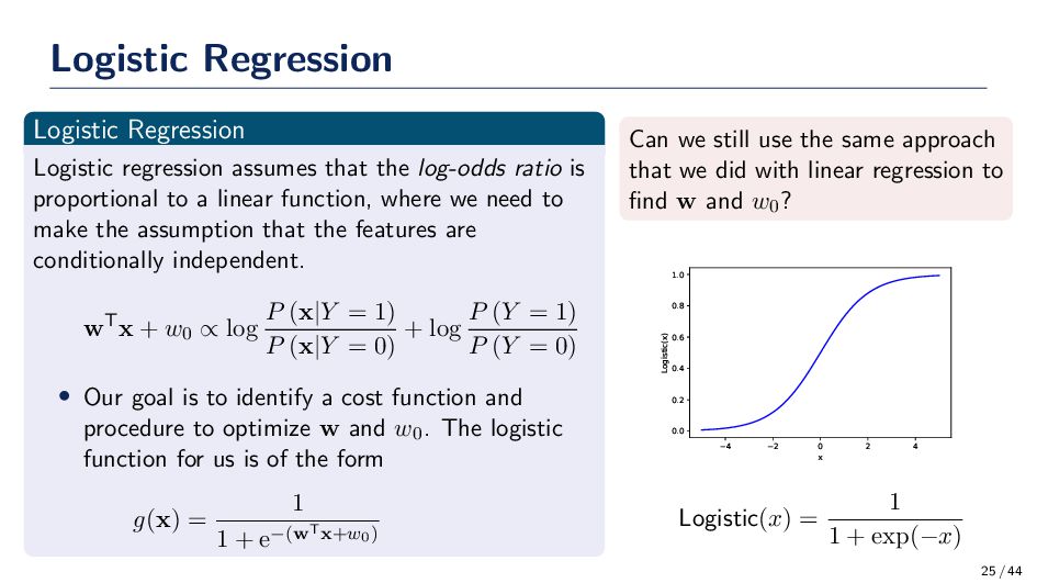
25. Logistic Regression Logistic Regression Logistic regression assumes that the log-odds ratio is proportional to a linear function, where we need to make the assumption that the features are conditionally independent. wTx + w0 ∝ log P (x|Y = 1) P (x|Y = 0) + log P (Y = 1) P (Y = 0) • Our goal is to identify a cost function and procedure to optimize w and w0. The logistic function for us is of the form g(x) = 1 1 + e−(wTx+w0) Can we still use the same approach that we did with linear regression to find w and w0? 4 2 0 2 4 x 0.0 0.2 0.4 0.6 0.8 1.0 Logistic(x) Logistic(x) = 1 1 + exp(−x) 25 / 44
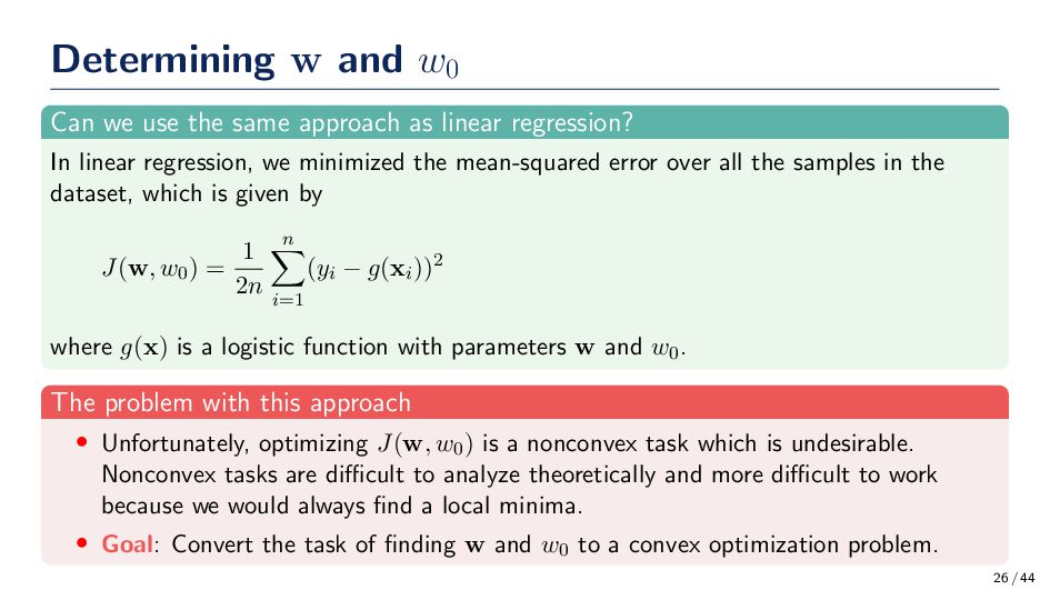
26. Determining w and w0 Can we use the same approach as linear regression? In linear regression, we minimized the mean-squared error over all the samples in the dataset, which is given by J(w, w0) = 1 2n n i=1 (yi − g(xi))2 where g(x) is a logistic function with parameters w and w0. The problem with this approach • Unfortunately, optimizing J(w, w0) is a nonconvex task which is undesirable. Nonconvex tasks are difficult to analyze theoretically and more difficult to work because we would always find a local minima. • Goal: Convert the task of finding w and w0 to a convex optimization problem. 26 / 44
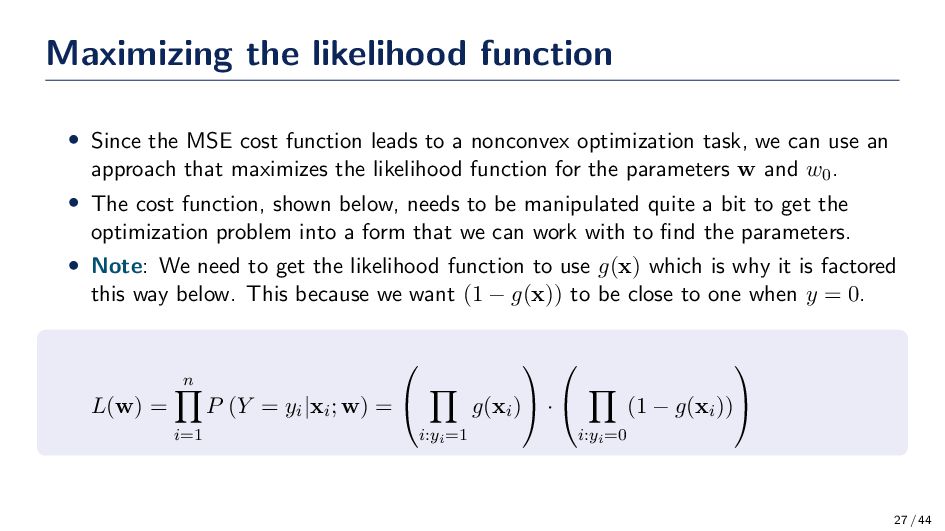
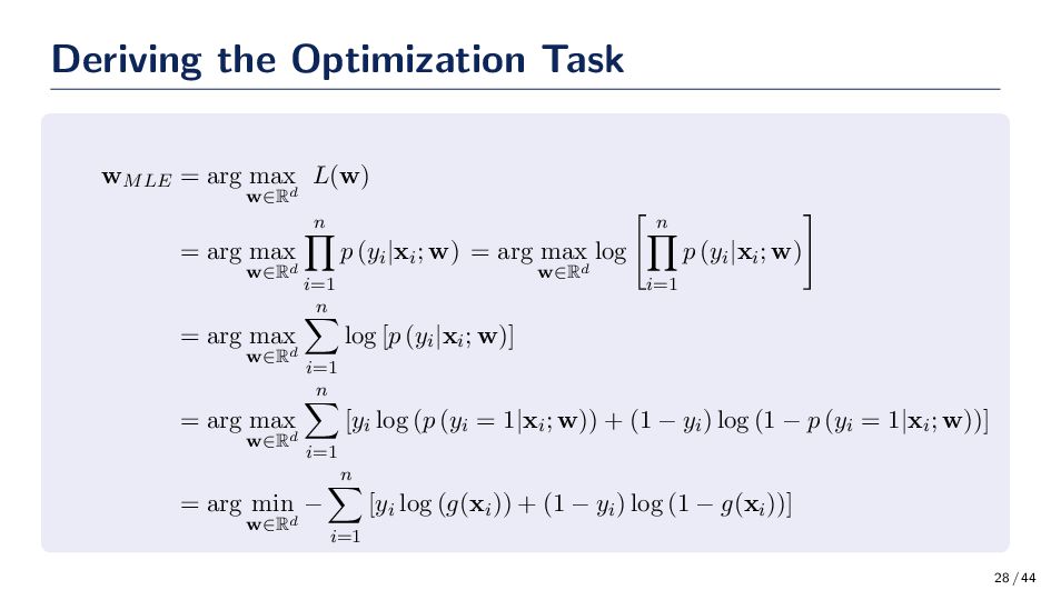
27. Maximizing the likelihood function • Since the MSE cost function leads to a nonconvex optimization task, we can use an approach that maximizes the likelihood function for the parameters w and w0. • The cost function, shown below, needs to be manipulated quite a bit to get the optimization problem into a form that we can work with to find the parameters. • Note: We need to get the likelihood function to use g(x) which is why it is factored this way below. This because we want (1 − g(x)) to be close to one when y = 0. L(w) = n i=1 P (Y = yi|xi; w) =   i:yi=1 g(xi)   ·   i:yi=0 (1 − g(xi))   27 / 44
28. Deriving the Optimization Task wMLE = arg max w∈Rd L(w) = arg max w∈Rd n i=1 p (yi|xi; w) = arg max w∈Rd log n i=1 p (yi|xi; w) = arg max w∈Rd n i=1 log [p (yi|xi; w)] = arg max w∈Rd n i=1 [yi log (p (yi = 1|xi; w)) + (1 − yi) log (1 − p (yi = 1|xi; w))] = arg min w∈Rd − n i=1 [yi log (g(xi)) + (1 − yi) log (1 − g(xi))] 28 / 44
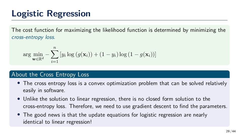
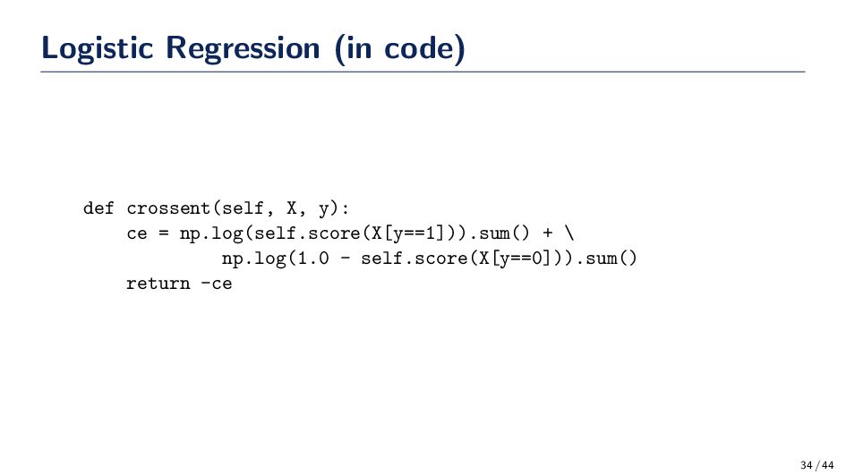
29. Logistic Regression The cost function for maximizing the likelihood function is determined by minimizing the cross-entropy loss. arg min w∈Rd − n i=1 [yi log (g(xi)) + (1 − yi) log (1 − g(xi))] About the Cross Entropy Loss • The cross entropy loss is a convex optimization problem that can be solved relatively easily in software. • Unlike the solution to linear regression, there is no closed form solution to the cross-entropy loss. Therefore, we need to use gradient descent to find the parameters. • The good news is that the update equations for logistic regression are nearly identical to linear regression! 29 / 44
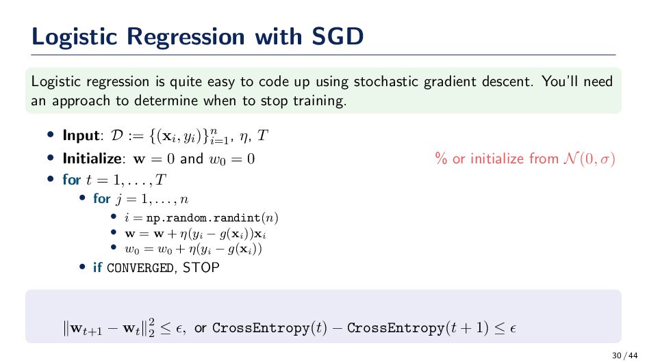
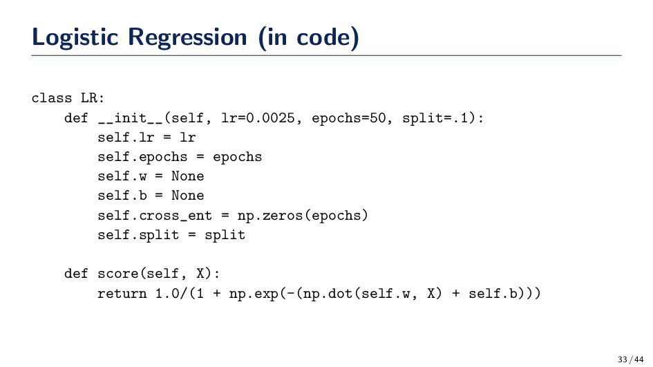
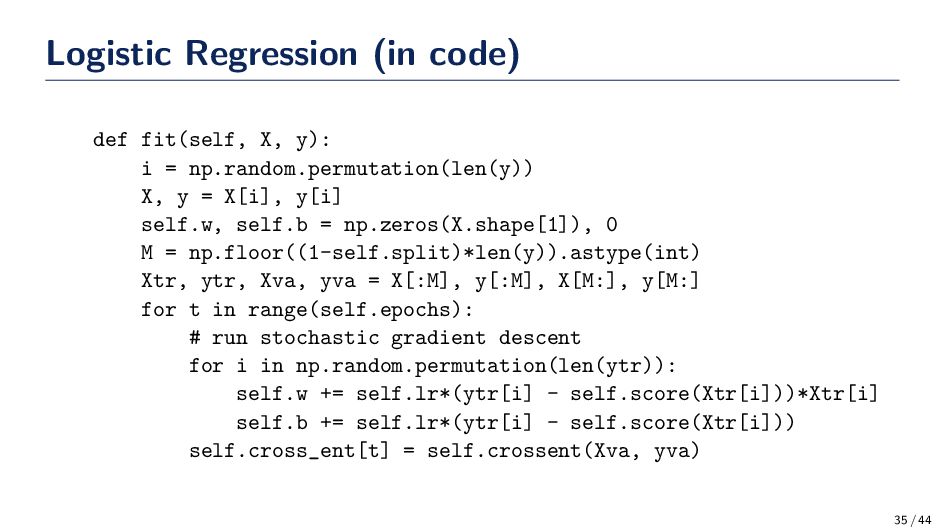
30. Logistic Regression with SGD Logistic regression is quite easy to code up using stochastic gradient descent. You’ll need an approach to determine when to stop training. • Input: D := {(xi, yi)}n i=1 , η, T • Initialize: w = 0 and w0 = 0 % or initialize from N(0, σ) • for t = 1, . . . , T • for j = 1, . . . , n • i = np.random.randint(n) • w = w + η(yi − g(xi ))xi • w0 = w0 + η(yi − g(xi )) • if CONVERGED, STOP ∥wt+1 − wt∥2 2 ≤ ϵ, or CrossEntropy(t) − CrossEntropy(t + 1) ≤ ϵ 30 / 44
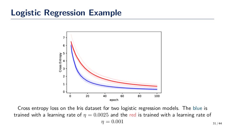
31. Logistic Regression Example 0 20 40 60 80 100 epoch 0 1 2 3 4 5 6 7 Cross Entropy Cross entropy loss on the Iris dataset for two logistic regression models. The blue is trained with a learning rate of η = 0.0025 and the red is trained with a learning rate of η = 0.001 31 / 44
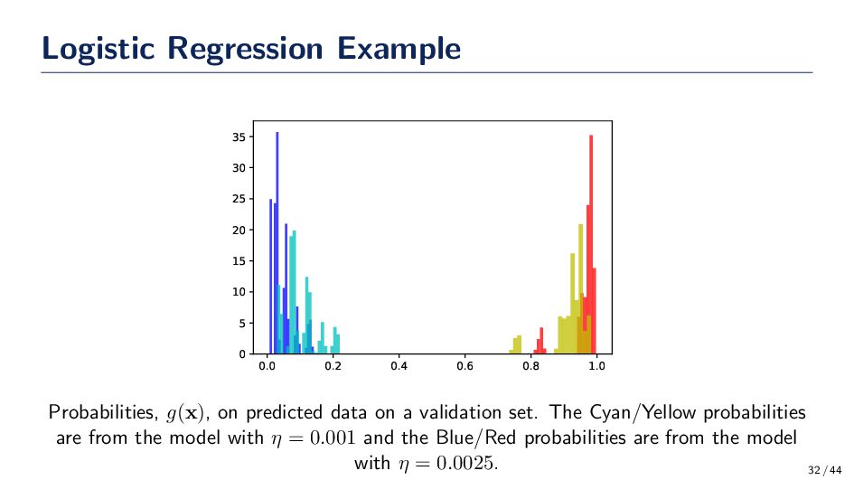
32. Logistic Regression Example 0.0 0.2 0.4 0.6 0.8 1.0 0 5 10 15 20 25 30 35 Probabilities, g(x), on predicted data on a validation set. The Cyan/Yellow probabilities are from the model with η = 0.001 and the Blue/Red probabilities are from the model with η = 0.0025. 32 / 44
33. Logistic Regression (in code) class LR: def __init__(self, lr=0.0025, epochs=50, split=.1): self.lr = lr self.epochs = epochs self.w = None self.b = None self.cross_ent = np.zeros(epochs) self.split = split def score(self, X): return 1.0/(1 + np.exp(-(np.dot(self.w, X) + self.b))) 33 / 44
34. Logistic Regression (in code) def crossent(self, X, y): ce = np.log(self.score(X[y==1])).sum() + \ np.log(1.0 - self.score(X[y==0])).sum() return -ce 34 / 44
35. Logistic Regression (in code) def fit(self, X, y): i = np.random.permutation(len(y)) X, y = X[i], y[i] self.w, self.b = np.zeros(X.shape[1]), 0 M = np.floor((1-self.split)*len(y)).astype(int) Xtr, ytr, Xva, yva = X[:M], y[:M], X[M:], y[M:] for t in range(self.epochs): # run stochastic gradient descent for i in np.random.permutation(len(ytr)): self.w += self.lr*(ytr[i] - self.score(Xtr[i]))*Xtr[i] self.b += self.lr*(ytr[i] - self.score(Xtr[i])) self.cross_ent[t] = self.crossent(Xva, yva) 35 / 44
36. Logistic Regression (in code) def predict(self, X): return 1.0*(self.score(X[i]) >= 0.5) def predict_proba(self, X): return self.score(X[i]) def predict_log_proba(self, X): return np.log(self.predict_proba(X)) 36 / 44
37. Multi-Class Scenarios 37 / 44
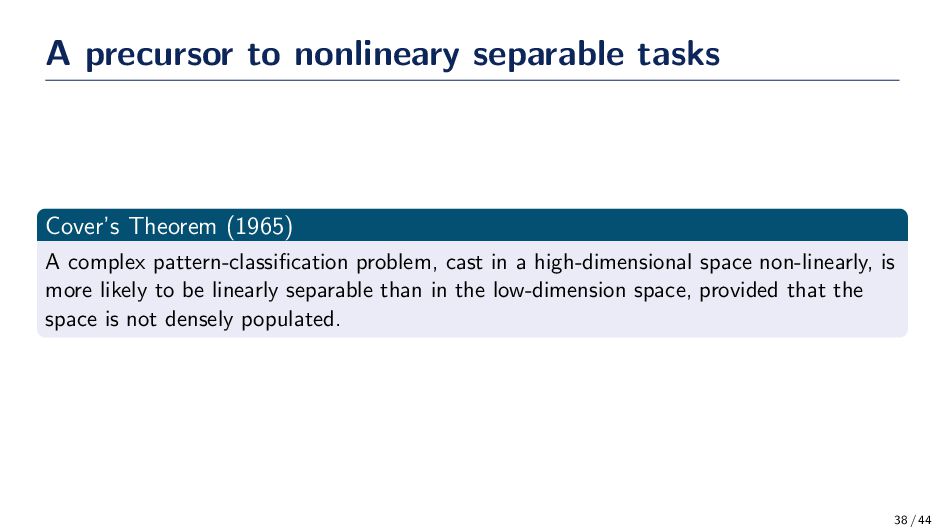
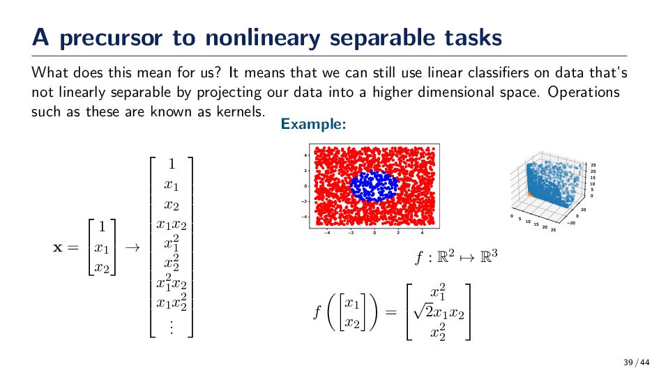
38. A precursor to nonlineary separable tasks Cover’s Theorem (1965) A complex pattern-classification problem, cast in a high-dimensional space non-linearly, is more likely to be linearly separable than in the low-dimension space, provided that the space is not densely populated. 38 / 44
39. A precursor to nonlineary separable tasks What does this mean for us? It means that we can still use linear classifiers on data that’s not linearly separable by projecting our data into a higher dimensional space. Operations such as these are known as kernels. x =   1 x1 x2   →                1 x1 x2 x1x2 x2 1 x2 2 x2 1 x2 x1x2 2 . . .                Example: 4 2 0 2 4 4 2 0 2 4 0 5 10 15 20 25 20 0 20 0 5 10 15 20 25 f : R2 → R3 f x1 x2 =   x2 1 √ 2x1x2 x2 2   39 / 44
40. A precursor to nonlineary separable tasks Note on a polynomial feature representation • Note that you can use the preprocessing function PolynomialFeatures in sklearn to implement this feature mapping. • It is also important to be aware that the dimensionality of the data can become extremely large by performing this operation. • In a later lecture, we will learn about how to use Cover’s theorem more efficiently when we discuss support vector machines (SVMs). 40 / 44
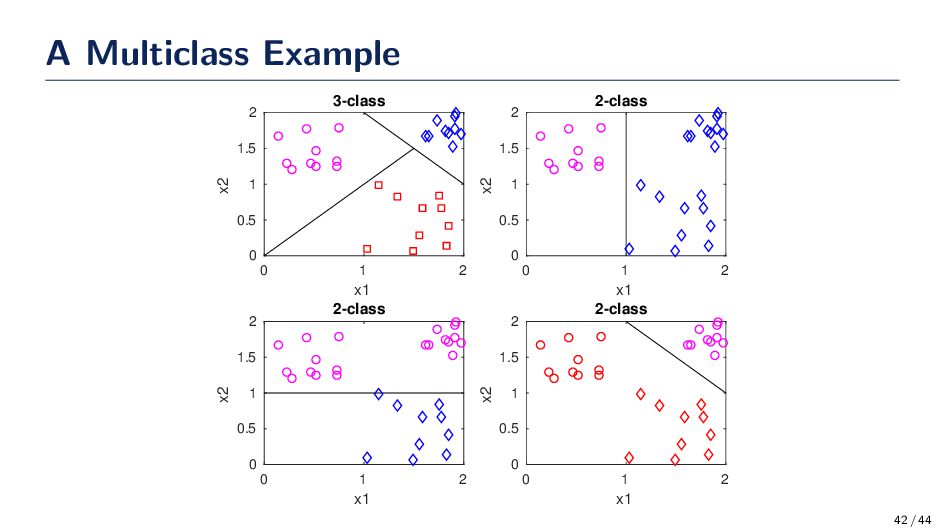
41. A Multiclass Example Note on a polynomial feature representation • All of the models presented so far are for two class problems. We need a way to extend these classification methods to multiple classes • Mathematically, this means that the class label, yi, for each datum is now yi ∈ {1, 2, ..., c}, where c is the number of possible classifications. Split the data into c two-class problems. • For example, if we have c classes then we will have c different classifiers: class 1 against classes {2, 3, ..., c}, class 2 against classes {1, 3, ..., c}, etc. Multiclass Prediction with Logistic Regression P(Y = k|x; w1, w2, · · · , wc) = exp(wT k x) c j=1 exp(wj Tx) 41 / 44
42. A Multiclass Example 0 1 2 x1 0 0.5 1 1.5 2 x2 3-class 0 1 2 x1 0 0.5 1 1.5 2 x2 2-class 0 1 2 x1 0 0.5 1 1.5 2 x2 2-class 0 1 2 x1 0 0.5 1 1.5 2 x2 2-class 42 / 44
43. Summary • This lecture introduces the concept of classification and regression for linear tasks. 43 / 44
44. The End 44 / 44