Machine Learning Lectures - Introduction

Transcript

1. Machine Learning Lectures Introduction to Machine Learning Gregory Ditzler gregory.ditzler@gmail.com February 24, 2024 1 / 49
2. Overview 1. Course Administration 2. Introduction to the Course 3. Background Material 4. Measuring Performance 2 / 49
3. Course Administration 3 / 49
4. About Me Gregory Ditzler Email: gregory.ditzler@gmail.com Web: http://gditzler.github.io Research Interests Incremental and online learning in nonstationary environments, adversarial machine learning, large-scale and distributed feature selection, applied machine learning 4 / 49
5. Breakdown of Grades • Homework • Approximately four or five assignments (theory + code) • Code must be submitted • Midterm Exams • Two exams • Final Project • Must be a (small) research project that is ideally aligned with your research • Rule of thumb: quality of a conference paper • A presentation is required. The talk will be 10-20 minutes, but more details will be covered closer to the end of the semester. • Groups of no more than two are allowed Check out the syllabus on Canvas for the exact breakdown of the grades. 5 / 49
6. Course Admin, Communication, etc. • This course will use Canvas (online.rowan.edu) for all course-related communication and file sharing. Please check Canvas regularly. Anything I say will be “posted” will show up on Canvas. • Communication: We will use the Canvas forums for course-related discussions. As students, you’re allowed (and encouraged) to post and reply to conversations. • Do not send me emails that are general to the class! Please use Canvas so everyone can see the response. • What was the trick to problem 2? I am getting an out-of-index error, what is wrong with my code? • Send me an email if you have a question(s) specific to you in the class. • I am worried about my grade. I am going to a conference on the day of the exam. . . 6 / 49
7. Textbooks References • “Introduction to Machine Learning” E. Alpaydin, MIT Press, 2014, 2nd Ed. [Free Online with IEEExplore] • “Elements of Statistical Learning Theory” T. Hastie, R. Tibshirani, and J. Friedman, Springer, 2008. [Free online] • “Deep Learning” I. Goodfellow, Y. Bengio and A. Courville, MIT Press, 2016. [Free online] • “Probabilistic Machine Learning: An Introduction,” K. Murphy, MIT Press, 2022. • “Pattern Recognition and Machine Learning,” C. Bishop, Springer 2006. [Free Online] 7 / 49
8. Software for Projects and Homework 8 / 49
9. Software for Projects and Homework 9 / 49
10. Did you see this article in the NYT? https://www.nytimes.com/2017/10/22/technology/ artificial-intelligence-experts-salaries.html 10 / 49
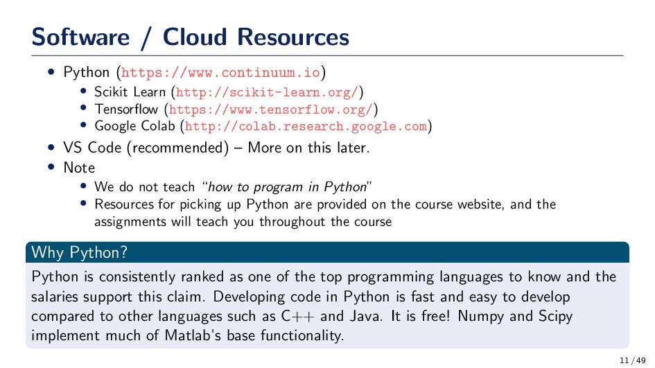
11. Software / Cloud Resources • Python (https://www.continuum.io) • Scikit Learn (http://scikit-learn.org/) • Tensorflow (https://www.tensorflow.org/) • Google Colab (http://colab.research.google.com) • VS Code (recommended) – More on this later. • Note • We do not teach “how to program in Python” • Resources for picking up Python are provided on the course website, and the assignments will teach you throughout the course Why Python? Python is consistently ranked as one of the top programming languages to know and the salaries support this claim. Developing code in Python is fast and easy to develop compared to other languages such as C++ and Java. It is free! Numpy and Scipy implement much of Matlab’s base functionality. 11 / 49
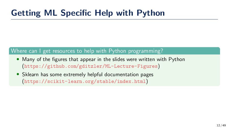
12. Getting ML Specific Help with Python Where can I get resources to help with Python programming? • Many of the figures that appear in the slides were written with Python (https://github.com/gditzler/ML-Lecture-Figures) • Sklearn has some extremely helpful documentation pages (https://scikit-learn.org/stable/index.html) 12 / 49
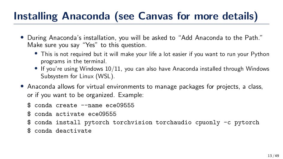
13. Installing Anaconda (see Canvas for more details) • During Anaconda’s installation, you will be asked to “Add Anaconda to the Path.” Make sure you say “Yes” to this question. • This is not required but it will make your life a lot easier if you want to run your Python programs in the terminal. • If you’re using Windows 10/11, you can also have Anaconda installed through Windows Subsystem for Linux (WSL). • Anaconda allows for virtual environments to manage packages for projects, a class, or if you want to be organized. Example: $ conda create --name ece09555 $ conda activate ece09555 $ conda install pytorch torchvision torchaudio cpuonly -c pytorch $ conda deactivate 13 / 49
14. Introduction to the Course 14 / 49
15. Contributors to ML 15 / 49
16. Text Prediction Given a word w(t) and some history h(t), what is the next word (i.e., w(t + 1))? What is the probability distribution over the next word (i.e., P(w(t + 1)|w(t), h(t)))? I love --? Can you pick up milk at the --? 16 / 49
17. Optical Character Recognition 17 / 49
18. Prediction of low/high risk loans savings income ✓1 ✓2 High-risk Low-risk +   +   +   +   +   +   +   -­‐   -­‐   -­‐   -­‐   -­‐   -­‐   -­‐   -­‐   -­‐   -­‐   -­‐   if (income > θ1 AND savings > θ2) then {low-risk} else {high-risk} 18 / 49
19. Finance 19 / 49
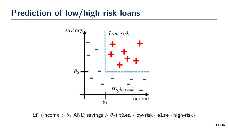
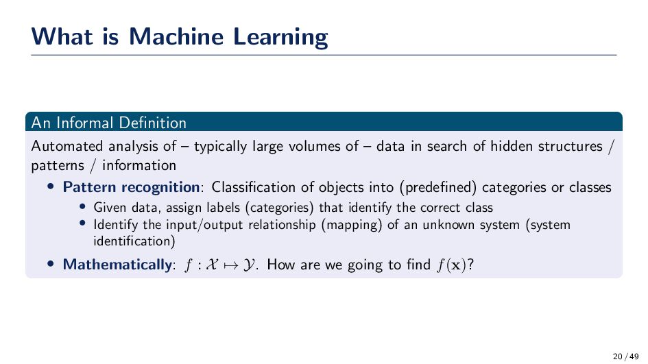
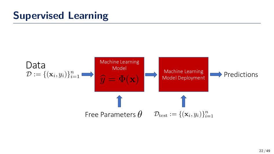
20. What is Machine Learning An Informal Definition Automated analysis of – typically large volumes of – data in search of hidden structures / patterns / information • Pattern recognition: Classification of objects into (predefined) categories or classes • Given data, assign labels (categories) that identify the correct class • Identify the input/output relationship (mapping) of an unknown system (system identification) • Mathematically: f : X → Y. How are we going to find f(x)? 20 / 49
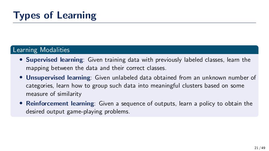
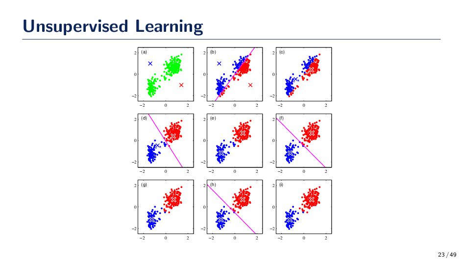
21. Types of Learning Learning Modalities • Supervised learning: Given training data with previously labeled classes, learn the mapping between the data and their correct classes. • Unsupervised learning: Given unlabeled data obtained from an unknown number of categories, learn how to group such data into meaningful clusters based on some measure of similarity • Reinforcement learning: Given a sequence of outputs, learn a policy to obtain the desired output game-playing problems. 21 / 49
22. Supervised Learning Data Machine Learning Model D := {(xi , yi )}n i=1 b y = (x) Dtest := {(xi , yi )}n i=1 Machine Learning Model Deployment Predictions Free Parameters ✓ 22 / 49
23. Unsupervised Learning (a) −2 0 2 −2 0 2 (b) −2 0 2 −2 0 2 (c) −2 0 2 −2 0 2 (d) −2 0 2 −2 0 2 (e) −2 0 2 −2 0 2 (f) −2 0 2 −2 0 2 (g) −2 0 2 −2 0 2 (h) −2 0 2 −2 0 2 (i) −2 0 2 −2 0 2 23 / 49
24. Reinforcement Learning 24 / 49
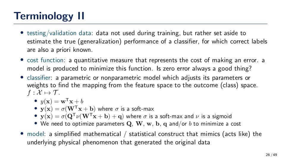
25. Terminology I • feature: a variable, x, believed to carry information about the task. example, cholesterol level. • feature vector: collection of variables, or features, x = [x1 , . . . , xD ]T. example, collection of medical tests for a patient. • feature space: D-dimensional vector space where the vectors x lie. example, x ∈ RD + • class: a category/value assigned to a feature vector. in general we can refer to this as the target variable (t). example, t = cancer or t = 10.2 ◦C. • pattern: a collection of features of an object under consideration, along with the correct class information of that object defined by, {xn , tn }. • training data: data used during training of a classifier for which the correct labels are a priori known. 25 / 49
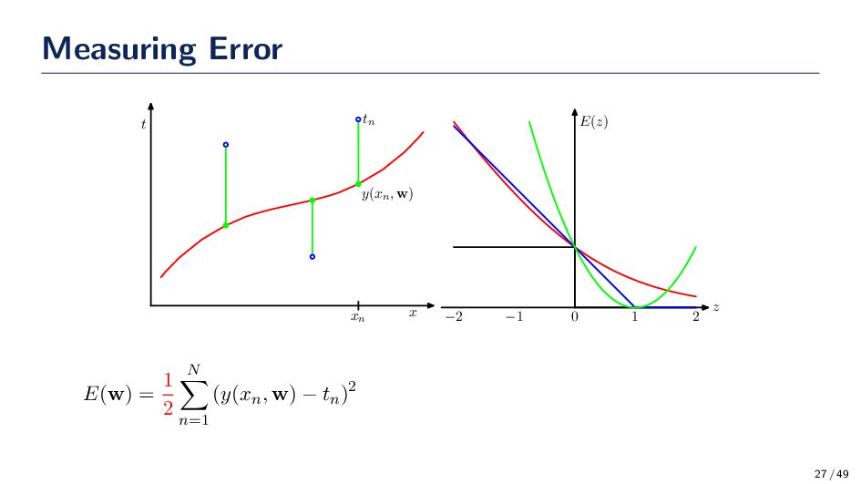
26. Terminology II • testing/validation data: data not used during training, but rather set aside to estimate the true (generalization) performance of a classifier, for which correct labels are also a priori known. • cost function: a quantitative measure that represents the cost of making an error. a model is produced to minimize this function. Is zero error always a good thing? • classifier: a parametric or nonparametric model which adjusts its parameters or weights to find the mapping from the feature space to the outcome (class) space. f : X → T . • y(x) = wTx + b • y(x) = σ(WTx + b) where σ is a soft-max • y(x) = σ(QTν(WTx + b) + q) where σ is a soft-max and ν is a sigmoid • We need to optimize parameters Q, W, w, b, q and/or b to minimize a cost • model: a simplified mathematical / statistical construct that mimics (acts like) the underlying physical phenomenon that generated the original data 26 / 49
27. Measuring Error t x y(xn , w) tn xn −2 −1 0 1 2 z E(z) E(w) = 1 2 N n=1 (y(xn , w) − tn )2 27 / 49
28. Overfitting y(x, w) = w0 + w1 x + w2 x2 + . . . + wM xM = M j=0 wj xj x t M = 0 0 1 −1 0 1 x t M = 1 0 1 −1 0 1 x t M = 3 0 1 −1 0 1 x t M = 9 0 1 −1 0 1 Bishop (2006) E(w) = 1 2 N n=1 (y(xn , w) − tn )2 , ERMS = 2E(w∗)/N 28 / 49
29. Overfitting y(x, w) = w0 + w1 x + w2 x2 + . . . + wM xM = M j=0 wj xj M ERMS 0 3 6 9 0 0.5 1 Training Test Bishop (2006) E(w) = 1 2 N n=1 (y(xn , w) − tn )2 , ERMS = 2E(w∗)/N 29 / 49
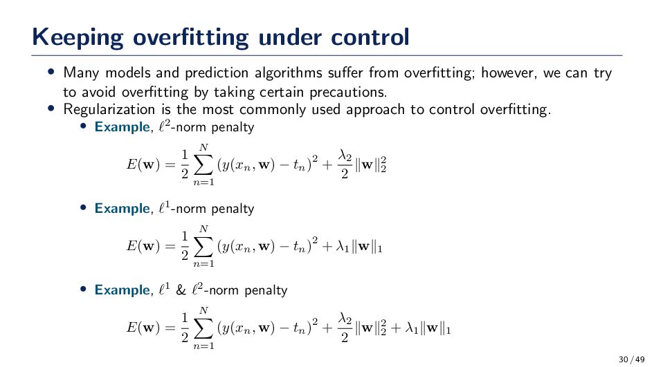
30. Keeping overfitting under control • Many models and prediction algorithms suffer from overfitting; however, we can try to avoid overfitting by taking certain precautions. • Regularization is the most commonly used approach to control overfitting. • Example, ℓ2-norm penalty E(w) = 1 2 N n=1 (y(xn , w) − tn )2 + λ2 2 ∥w∥2 2 • Example, ℓ1-norm penalty E(w) = 1 2 N n=1 (y(xn , w) − tn )2 + λ1 ∥w∥1 • Example, ℓ1 & ℓ2-norm penalty E(w) = 1 2 N n=1 (y(xn , w) − tn )2 + λ2 2 ∥w∥2 2 + λ1 ∥w∥1 30 / 49
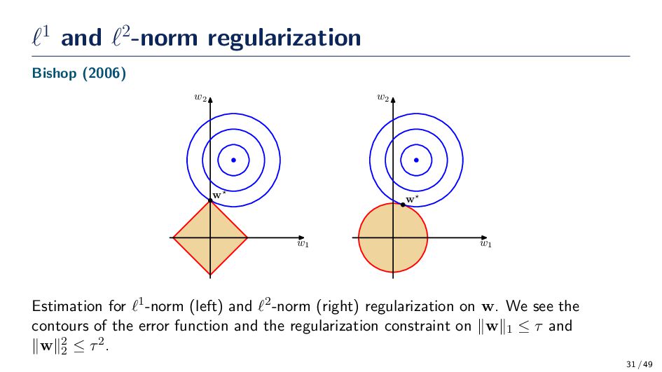
31. ℓ1 and ℓ2-norm regularization Bishop (2006) w1 w2 w w1 w2 w Estimation for ℓ1-norm (left) and ℓ2-norm (right) regularization on w. We see the contours of the error function and the regularization constraint on ∥w∥1 ≤ τ and ∥w∥2 2 ≤ τ2. 31 / 49
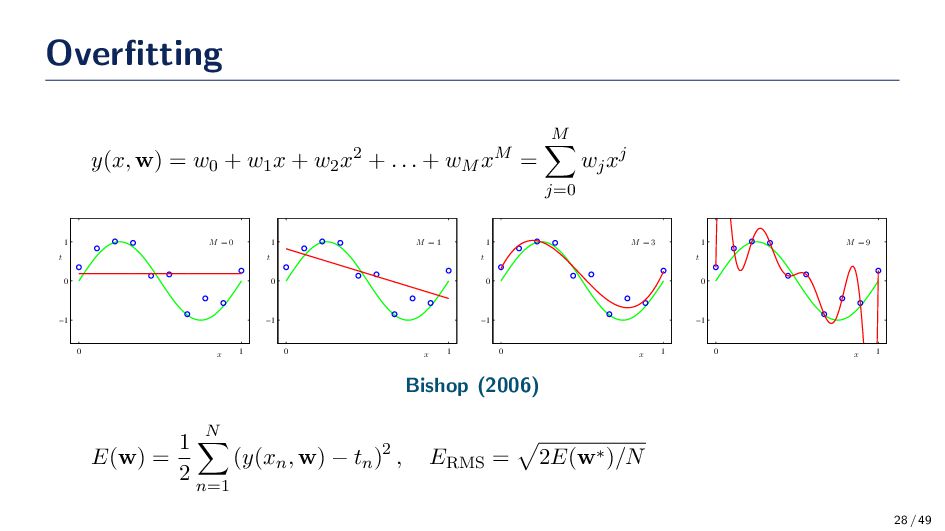
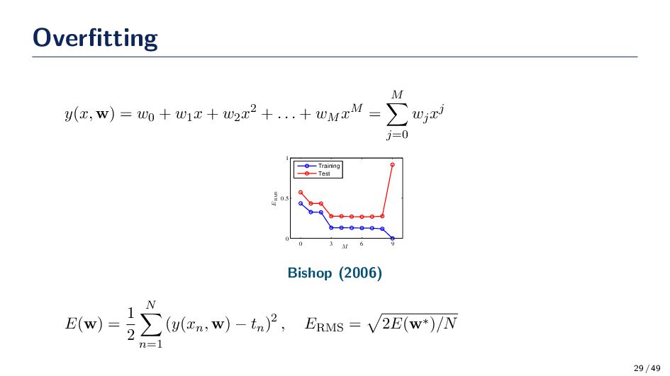
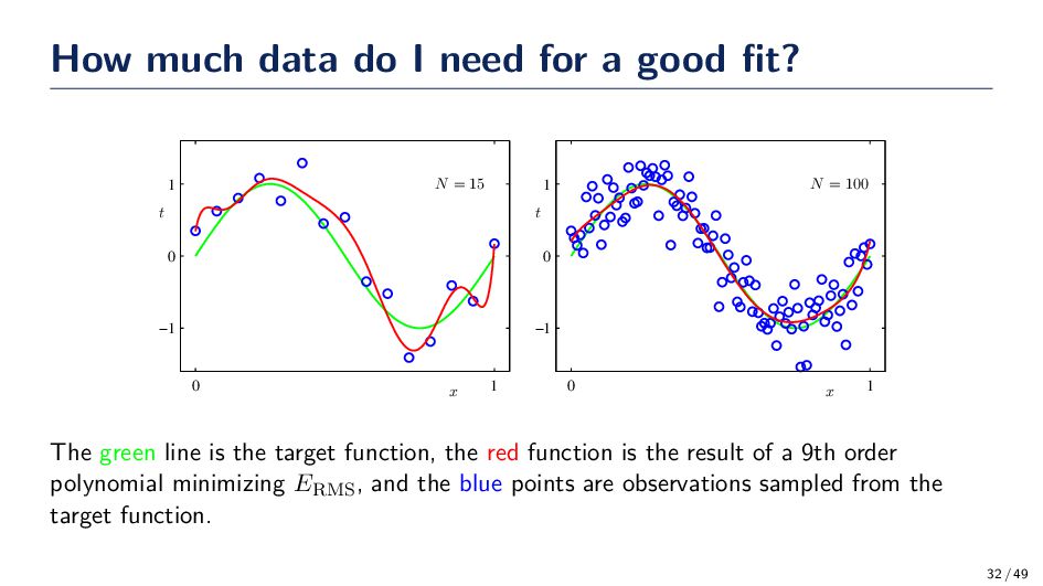
32. How much data do I need for a good fit? x t N = 15 0 1 −1 0 1 x t N = 100 0 1 −1 0 1 The green line is the target function, the red function is the result of a 9th order polynomial minimizing ERMS, and the blue points are observations sampled from the target function. 32 / 49
33. Background Material 33 / 49
34. Bayes Decision Theory Probability Theory • Pattern recognition requires that we have a way to deal with uncertainty, which arises from noise in data and finite sample sizes. Three things in life are certain: (1) death, (2) taxes, and (3) noise in your data! • Some definitions • Evidence: The probability of making such an observation. • Prior: Our degree of belief that the event is plausible in the first place • Likelihood: The likelihood of making an observation, under the condition that the event has occurred. Let us define some notation. Let X and Y be random variables. For example, X is a collection of medical measurements and Y is the healthy/unhealthy. Recall that there are three axioms of probability that must hold: P(E) = 1, P(E) ≥ 0 ∀E ∈ E, P (∪n i=1 Ei ) = n i=1 P(Ei ) 34 / 49
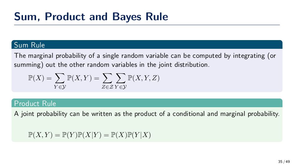
35. Sum, Product and Bayes Rule Sum Rule The marginal probability of a single random variable can be computed by integrating (or summing) out the other random variables in the joint distribution. P(X) = Y ∈Y P(X, Y ) = Z∈Z Y ∈Y P(X, Y, Z) Product Rule A joint probability can be written as the product of a conditional and marginal probability. P(X, Y ) = P(Y )P(X|Y ) = P(X)P(Y |X) 35 / 49
36. Sum, Product and Bayes Rule Bayes Rule A simple manipulation of the product rule gives rise to the Bayes rule. P(Y |X) = P(Y )P(X|Y ) P(X) = P(Y )P(X|Y ) Y ∈Y P(X, Y ) = P(Y )P(X|Y ) Y ′∈Y P(Y ′)P(X|Y ′) 36 / 49
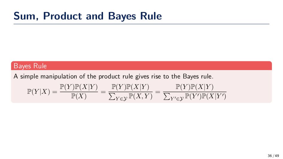
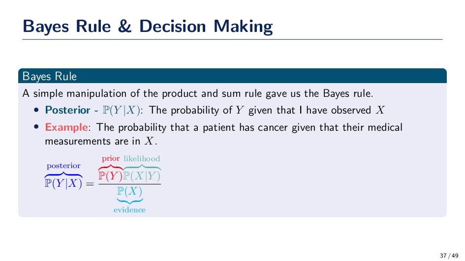
37. Bayes Rule & Decision Making Bayes Rule A simple manipulation of the product and sum rule gave us the Bayes rule. • Posterior - P(Y |X): The probability of Y given that I have observed X • Example: The probability that a patient has cancer given that their medical measurements are in X. posterior P(Y |X) = prior P(Y ) likelihood P(X|Y ) P(X) evidence 37 / 49
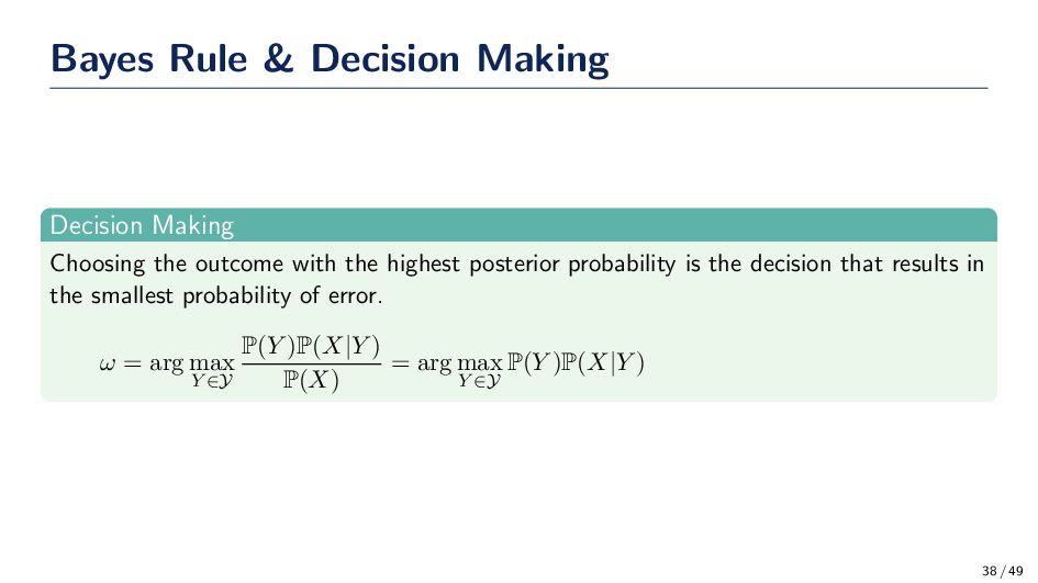
38. Bayes Rule & Decision Making Decision Making Choosing the outcome with the highest posterior probability is the decision that results in the smallest probability of error. ω = arg max Y ∈Y P(Y )P(X|Y ) P(X) = arg max Y ∈Y P(Y )P(X|Y ) 38 / 49
39. Measuring Performance 39 / 49
40. Cross Validation Divide the data into k disjoint sets. The train on k − 1 sets and test of the kth. The process of cross-validation produces k error estimates. block 1 block 2 block 3 . . . . . . block k − 1 block k block 1 block 2 block 3 . . . . . . block k − 1 block k ϵ1 block 1 block 2 block 3 . . . . . . block k − 1 block k ϵ2 . . . block 1 block 2 block 3 . . . . . . block k − 1 block k ϵk−2 block 1 block 2 block 3 . . . . . . block k − 1 block k ϵk−1 block 1 block 2 block 3 . . . . . . block k − 1 block k ϵk The k-fold CV error is given by: err = 1 k k i=1 ϵk Refer to Demˇ sar’s JMLR (2006) article on comparing multiple classifiers. 40 / 49
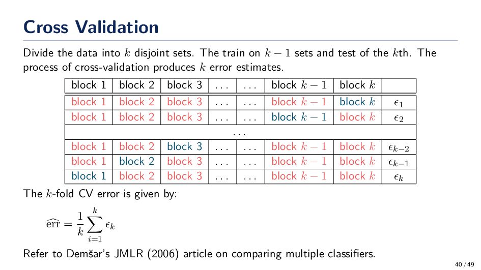
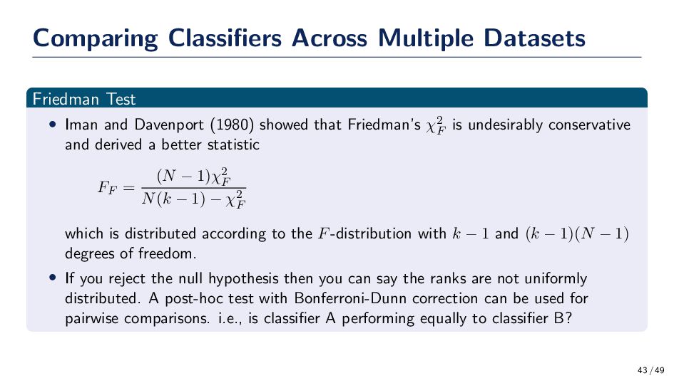
41. Comparing Classifiers Across Multiple Datasets Demˇ sar, JMLR (2006) • What if we want to benchmark a new algorithm against the state-of-the-art? How should we determine if there is significance in the results? • Confidence intervals: This works OK if we have one dataset and one other classifier. What if we have multiple classifiers and multiple datasets? • Confidence intervals are not always useful. Think about it. . . We might not have significance at 5-fold, but we do at 500-fold. CI = x ± 1.96σ/ √ n • The Friedman test is a robust rank-based hypothesis test to compare multiple classifiers across multiple datasets. • Null hypothesis: All classifiers are performing equally well. Janez Demˇ sar, “Statistical Comparisons of Classifiers over Multiple Data Sets,” Journal of Machine Learning Research, vol. 7, 2006, pp. 1–30. 41 / 49
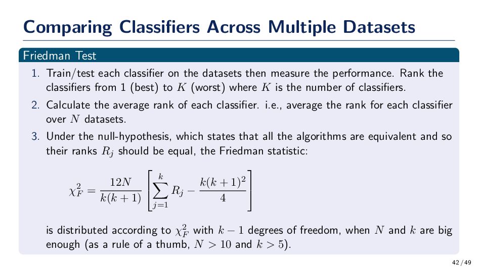
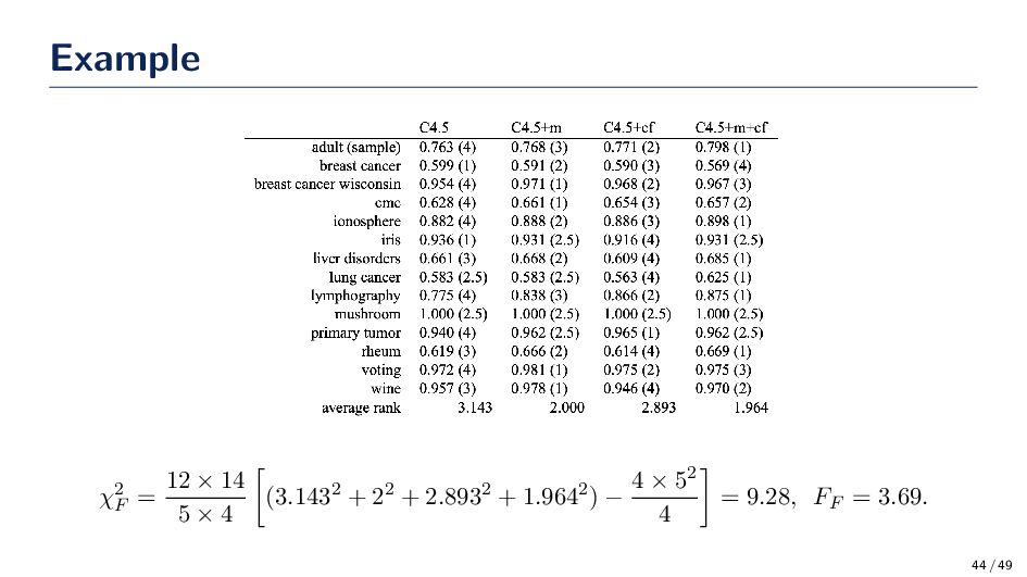
42. Comparing Classifiers Across Multiple Datasets Friedman Test 1. Train/test each classifier on the datasets then measure the performance. Rank the classifiers from 1 (best) to K (worst) where K is the number of classifiers. 2. Calculate the average rank of each classifier. i.e., average the rank for each classifier over N datasets. 3. Under the null-hypothesis, which states that all the algorithms are equivalent and so their ranks Rj should be equal, the Friedman statistic: χ2 F = 12N k(k + 1)   k j=1 Rj − k(k + 1)2 4   is distributed according to χ2 F with k − 1 degrees of freedom, when N and k are big enough (as a rule of a thumb, N > 10 and k > 5). 42 / 49
43. Comparing Classifiers Across Multiple Datasets Friedman Test • Iman and Davenport (1980) showed that Friedman’s χ2 F is undesirably conservative and derived a better statistic FF = (N − 1)χ2 F N(k − 1) − χ2 F which is distributed according to the F-distribution with k − 1 and (k − 1)(N − 1) degrees of freedom. • If you reject the null hypothesis then you can say the ranks are not uniformly distributed. A post-hoc test with Bonferroni-Dunn correction can be used for pairwise comparisons. i.e., is classifier A performing equally to classifier B? 43 / 49
44. Example χ2 F = 12 × 14 5 × 4 (3.1432 + 22 + 2.8932 + 1.9642) − 4 × 52 4 = 9.28, FF = 3.69. 44 / 49
45. Figures of Merit Confusion Matrix true + − predicted + TP FP − FN TN Some commonly used figures of merit: recall = TP TP + FP , precision = TP TP + FN , f-measure = 2 × precision × recall precision + recall Receiver operating characteristic (ROC) curves are used to show the trade off between true positive and false positive rates. 45 / 49
46. Confusion Matrices 0 1 Predicted label 0 1 True label 12 1 2 10 2 4 6 8 10 12 46 / 49
47. Receiver operating characteristic (ROC) curve 0.0 0.2 0.4 0.6 0.8 1.0 False Positive Rate 0.0 0.2 0.4 0.6 0.8 1.0 True Positive Rate micro-average ROC curve (area = 0.73) macro-average ROC curve (area = 0.78) ROC curve of class 0 (area = 0.91) ROC curve of class 1 (area = 0.60) ROC curve of class 2 (area = 0.79) Tom Fawcett, “An introduction to ROC analysis,” Pattern Recognition Letters Volume 27, Issue 8, June 2006, Pages 861-874. 47 / 49
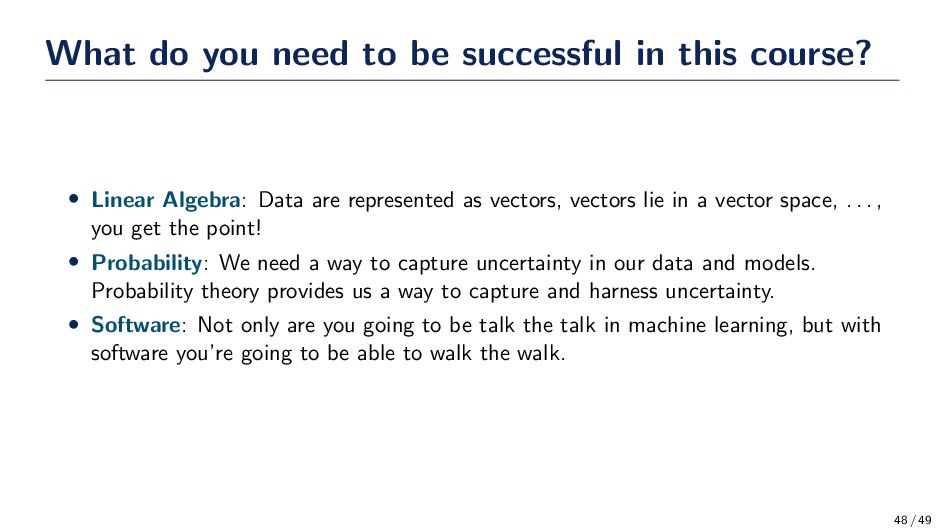
48. What do you need to be successful in this course? • Linear Algebra: Data are represented as vectors, vectors lie in a vector space, . . . , you get the point! • Probability: We need a way to capture uncertainty in our data and models. Probability theory provides us a way to capture and harness uncertainty. • Software: Not only are you going to be talk the talk in machine learning, but with software you’re going to be able to walk the walk. 48 / 49
49. The End 49 / 49