Machine Learning Lectures - Support Vector Machines

Transcript

1. Machine Learning Lectures Support Vector Machines Gregory Ditzler gregory.ditzler@gmail.com February 24, 2024 1 / 40
2. Overview 1. Motivation and Setup 2. The Hard Margin SVM 3. The Soft Margin SVM 4. Sequential Minimal Optimization 5. Kernels 2 / 40
3. Motivation and Setup 3 / 40
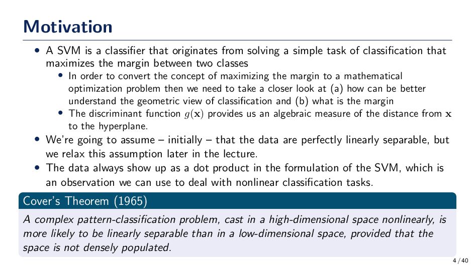
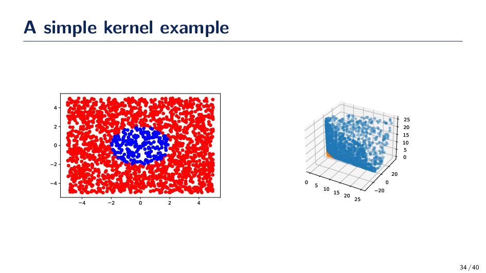
4. Motivation • A SVM is a classifier that originates from solving a simple task of classification that maximizes the margin between two classes • In order to convert the concept of maximizing the margin to a mathematical optimization problem then we need to take a closer look at (a) how can be better understand the geometric view of classification and (b) what is the margin • The discriminant function g(x) provides us an algebraic measure of the distance from x to the hyperplane. • We’re going to assume – initially – that the data are perfectly linearly separable, but we relax this assumption later in the lecture. • The data always show up as a dot product in the formulation of the SVM, which is an observation we can use to deal with nonlinear classification tasks. Cover’s Theorem (1965) A complex pattern-classification problem, cast in a high-dimensional space nonlinearly, is more likely to be linearly separable than in a low-dimensional space, provided that the space is not densely populated. 4 / 40
5. The SVM and Linear Classification R+ R− xp H wTx + b > 1 g(x) = wTx + b = 0 wTx + b < −1 M argin r w 5 / 40
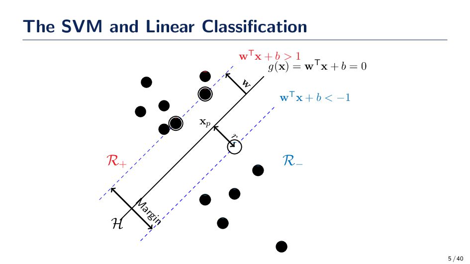
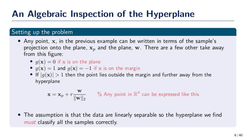
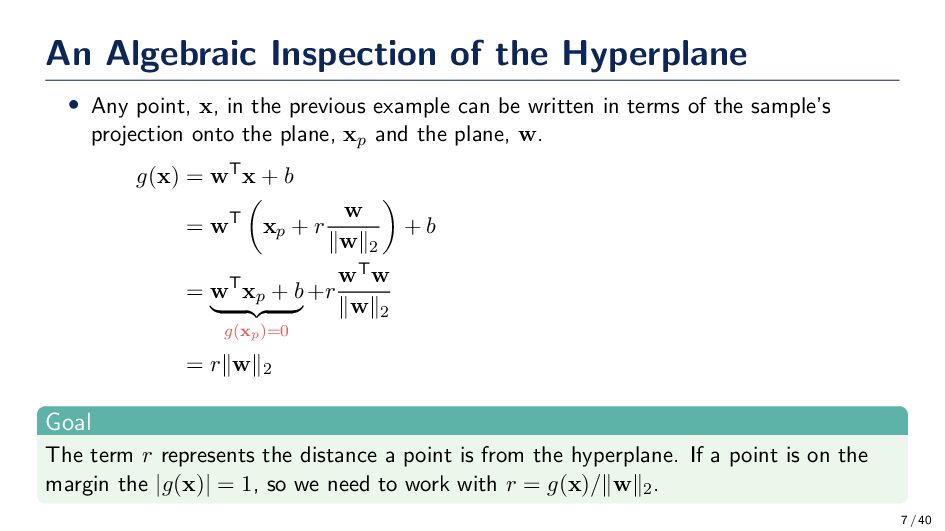
6. An Algebraic Inspection of the Hyperplane Setting up the problem • Any point, x, in the previous example can be written in terms of the sample’s projection onto the plane, xp and the plane, w. There are a few other take away from this figure: • g(x) = 0 if x is on the plane • g(x) = 1 and g(x) = −1 if x is on the margin • If |g(x)| > 1 then the point lies outside the margin and further away from the hyperplane x = xp + r w ∥w∥2 % Any point in Rd can be expressed like this • The assumption is that the data are linearly separable so the hyperplane we find must classify all the samples correctly. 6 / 40
7. An Algebraic Inspection of the Hyperplane • Any point, x, in the previous example can be written in terms of the sample’s projection onto the plane, xp and the plane, w. g(x) = wTx + b = wT xp + r w ∥w∥2 + b = wTxp + b g(xp)=0 +r wTw ∥w∥2 = r∥w∥2 Goal The term r represents the distance a point is from the hyperplane. If a point is on the margin the |g(x)| = 1, so we need to work with r = g(x)/∥w∥2. 7 / 40
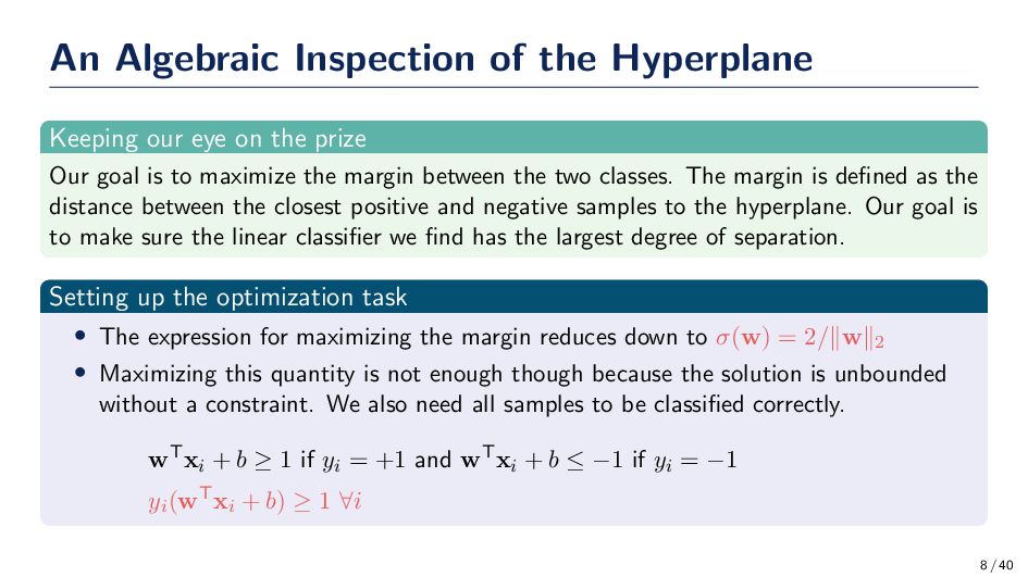
8. An Algebraic Inspection of the Hyperplane Keeping our eye on the prize Our goal is to maximize the margin between the two classes. The margin is defined as the distance between the closest positive and negative samples to the hyperplane. Our goal is to make sure the linear classifier we find has the largest degree of separation. Setting up the optimization task • The expression for maximizing the margin reduces down to σ(w) = 2/∥w∥2 • Maximizing this quantity is not enough though because the solution is unbounded without a constraint. We also need all samples to be classified correctly. wTxi + b ≥ 1 if yi = +1 and wTxi + b ≤ −1 if yi = −1 yi(wTxi + b) ≥ 1 ∀i 8 / 40
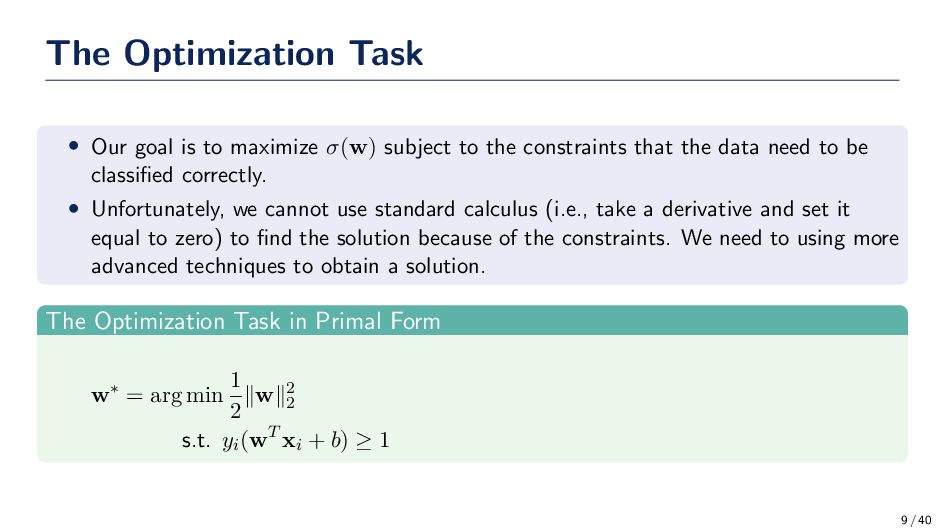
9. The Optimization Task • Our goal is to maximize σ(w) subject to the constraints that the data need to be classified correctly. • Unfortunately, we cannot use standard calculus (i.e., take a derivative and set it equal to zero) to find the solution because of the constraints. We need to using more advanced techniques to obtain a solution. The Optimization Task in Primal Form w∗ = arg min 1 2 ∥w∥2 2 s.t. yi(wT xi + b) ≥ 1 9 / 40
10. The Hard Margin SVM 10 / 40
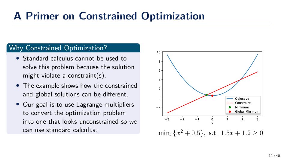
11. A Primer on Constrained Optimization Why Constrained Optimization? • Standard calculus cannot be used to solve this problem because the solution might violate a constraint(s). • The example shows how the constrained and global solutions can be different. • Our goal is to use Lagrange multipliers to convert the optimization problem into one that looks unconstrained so we can use standard calculus. 3 2 1 0 1 2 3 x 2 0 2 4 6 8 10 Objective Constraint Minimum Global Minimum minx{x2 + 0.5}, s.t. 1.5x + 1.2 ≥ 0 11 / 40
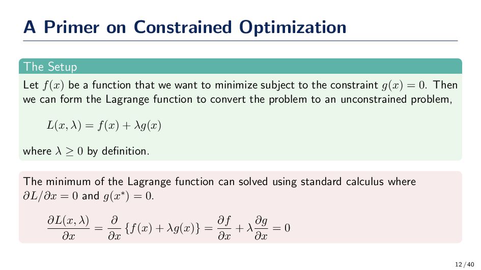
12. A Primer on Constrained Optimization The Setup Let f(x) be a function that we want to minimize subject to the constraint g(x) = 0. Then we can form the Lagrange function to convert the problem to an unconstrained problem, L(x, λ) = f(x) + λg(x) where λ ≥ 0 by definition. The minimum of the Lagrange function can solved using standard calculus where ∂L/∂x = 0 and g(x∗) = 0. ∂L(x, λ) ∂x = ∂ ∂x {f(x) + λg(x)} = ∂f ∂x + λ ∂g ∂x = 0 12 / 40
13. A Primer on Constrained Optimization • Our problem is slightly different than the generic example since we have n constraints not one. Therefore, we’re going to have n Lagrange multipliers (i.e., one for each constraint). • We still need to require that ∂L/∂x = 0 even when there are n constraints, so this approach of using Lagrange multipliers can generalize to out problem. 13 / 40
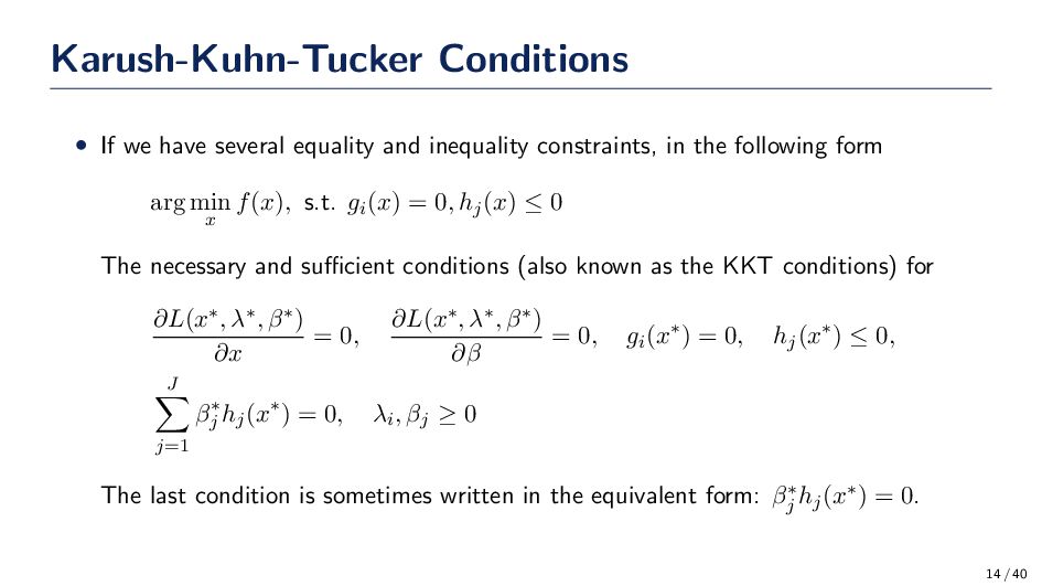
14. Karush-Kuhn-Tucker Conditions • If we have several equality and inequality constraints, in the following form arg min x f(x), s.t. gi(x) = 0, hj(x) ≤ 0 The necessary and sufficient conditions (also known as the KKT conditions) for ∂L(x∗, λ∗, β∗) ∂x = 0, ∂L(x∗, λ∗, β∗) ∂β = 0, gi(x∗) = 0, hj(x∗) ≤ 0, J j=1 β∗ j hj(x∗) = 0, λi, βj ≥ 0 The last condition is sometimes written in the equivalent form: β∗ j hj(x∗) = 0. 14 / 40
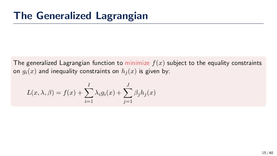
15. The Generalized Lagrangian The generalized Lagrangian function to minimize f(x) subject to the equality constraints on gi(x) and inequality constraints on hj(x) is given by: L(x, λ, β) = f(x) + I i=1 λigi(x) + J j=1 βjhj(x) 15 / 40
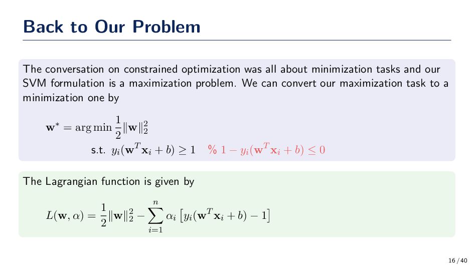
16. Back to Our Problem The conversation on constrained optimization was all about minimization tasks and our SVM formulation is a maximization problem. We can convert our maximization task to a minimization one by w∗ = arg min 1 2 ∥w∥2 2 s.t. yi(wT xi + b) ≥ 1 % 1 − yi(wT xi + b) ≤ 0 The Lagrangian function is given by L(w, α) = 1 2 ∥w∥2 2 − n i=1 αi yi(wT xi + b) − 1 16 / 40
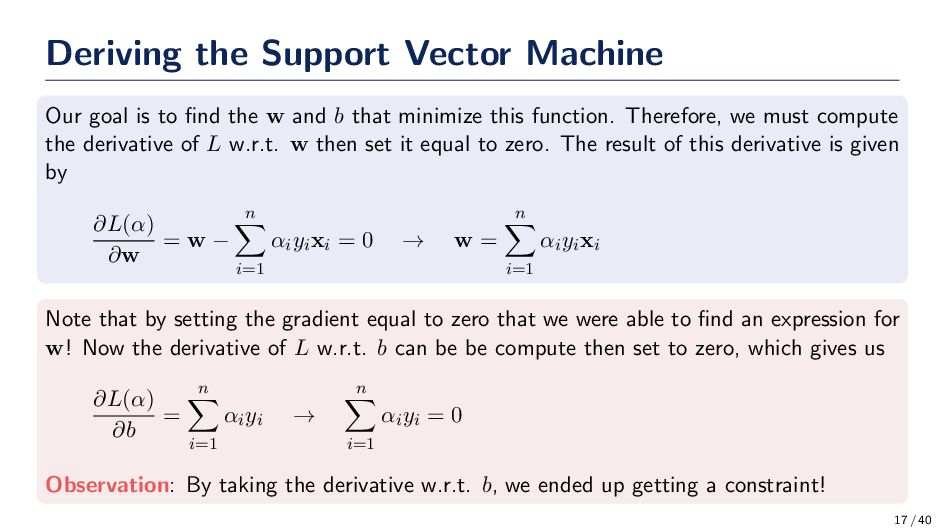
17. Deriving the Support Vector Machine Our goal is to find the w and b that minimize this function. Therefore, we must compute the derivative of L w.r.t. w then set it equal to zero. The result of this derivative is given by ∂L(α) ∂w = w − n i=1 αiyixi = 0 → w = n i=1 αiyixi Note that by setting the gradient equal to zero that we were able to find an expression for w! Now the derivative of L w.r.t. b can be be compute then set to zero, which gives us ∂L(α) ∂b = n i=1 αiyi → n i=1 αiyi = 0 Observation: By taking the derivative w.r.t. b, we ended up getting a constraint! 17 / 40
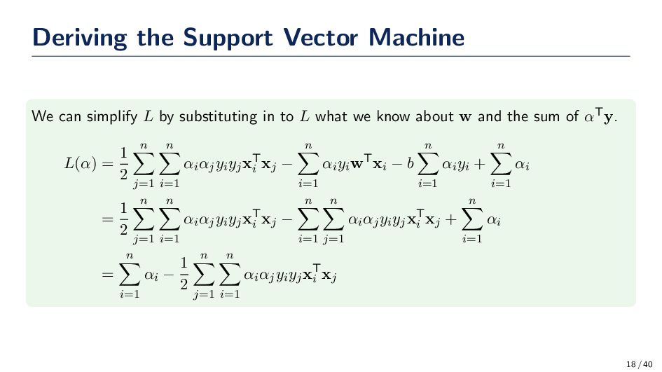
18. Deriving the Support Vector Machine We can simplify L by substituting in to L what we know about w and the sum of αTy. L(α) = 1 2 n j=1 n i=1 αiαjyiyjxT i xj − n i=1 αiyiwTxi − b n i=1 αiyi + n i=1 αi = 1 2 n j=1 n i=1 αiαjyiyjxT i xj − n i=1 n j=1 αiαjyiyjxT i xj + n i=1 αi = n i=1 αi − 1 2 n j=1 n i=1 αiαjyiyjxT i xj 18 / 40
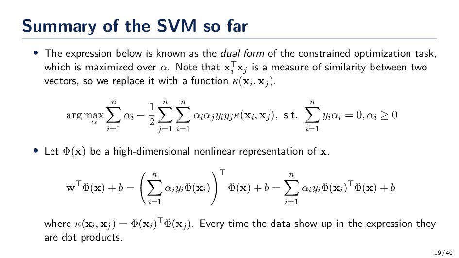
19. Summary of the SVM so far • The expression below is known as the dual form of the constrained optimization task, which is maximized over α. Note that xT i xj is a measure of similarity between two vectors, so we replace it with a function κ(xi, xj). arg max α n i=1 αi − 1 2 n j=1 n i=1 αiαjyiyjκ(xi, xj), s.t. n i=1 yiαi = 0, αi ≥ 0 • Let Φ(x) be a high-dimensional nonlinear representation of x. wTΦ(x) + b = n i=1 αiyiΦ(xi) T Φ(x) + b = n i=1 αiyiΦ(xi)TΦ(x) + b where κ(xi, xj) = Φ(xi)TΦ(xj). Every time the data show up in the expression they are dot products. 19 / 40
20. The Soft Margin SVM 20 / 40
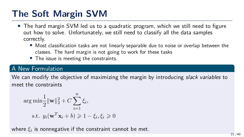
21. The Soft Margin SVM • The hard margin SVM led us to a quadratic program, which we still need to figure out how to solve. Unfortunately, we still need to classify all the data samples correctly. • Most classification tasks are not linearly separable due to noise or overlap between the classes. The hard margin is not going to work for these tasks • The issue is meeting the constraints. A New Formulation We can modify the objective of maximizing the margin by introducing slack variables to meet the constraints arg min 1 2 ∥w∥2 2 + C n i=1 ξi, s.t. yi(wT xi + b) ⩾ 1 − ξi, ξi ⩾ 0 where ξi is nonnegative if the constraint cannot be met. 21 / 40
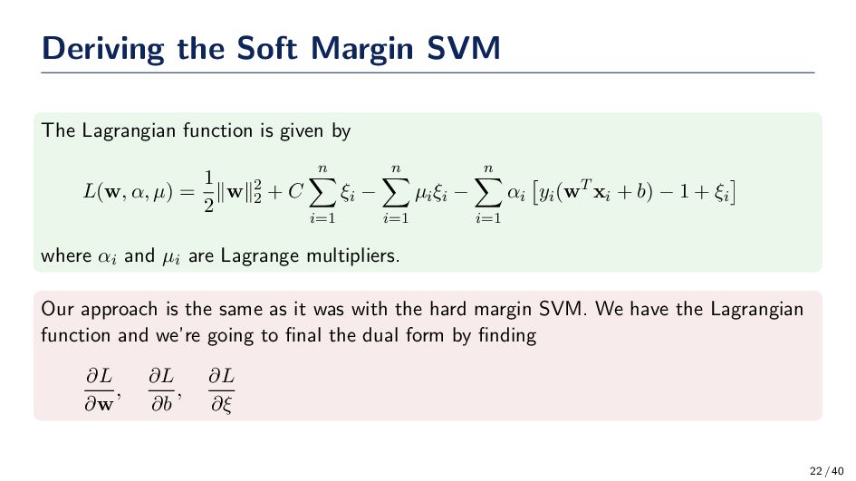
22. Deriving the Soft Margin SVM The Lagrangian function is given by L(w, α, µ) = 1 2 ∥w∥2 2 + C n i=1 ξi − n i=1 µiξi − n i=1 αi yi(wT xi + b) − 1 + ξi where αi and µi are Lagrange multipliers. Our approach is the same as it was with the hard margin SVM. We have the Lagrangian function and we’re going to final the dual form by finding ∂L ∂w , ∂L ∂b , ∂L ∂ξ 22 / 40
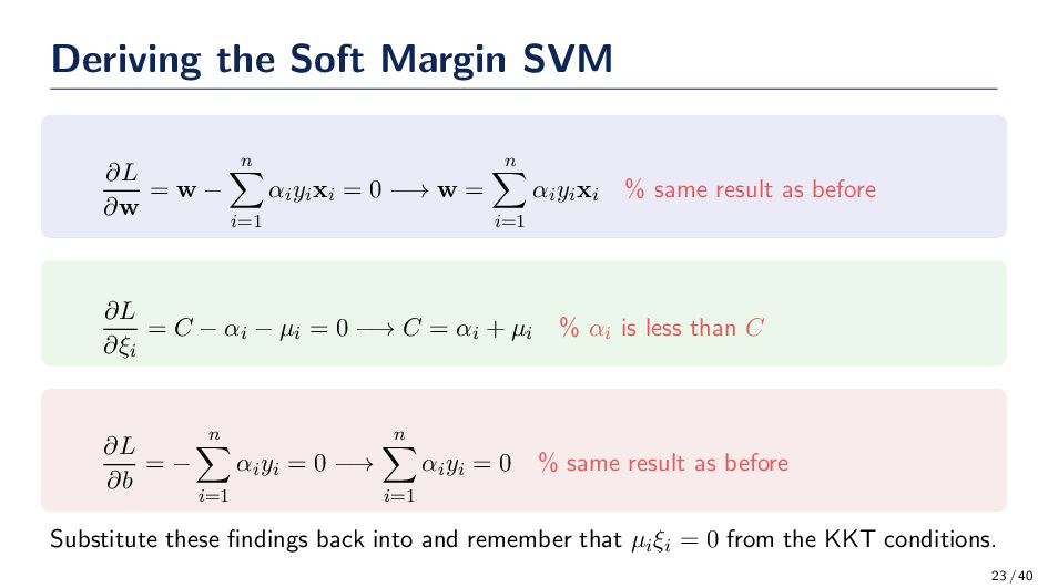
23. Deriving the Soft Margin SVM ∂L ∂w = w − n i=1 αiyixi = 0 −→ w = n i=1 αiyixi % same result as before ∂L ∂ξi = C − αi − µi = 0 −→ C = αi + µi % αi is less than C ∂L ∂b = − n i=1 αiyi = 0 −→ n i=1 αiyi = 0 % same result as before Substitute these findings back into and remember that µiξi = 0 from the KKT conditions. 23 / 40
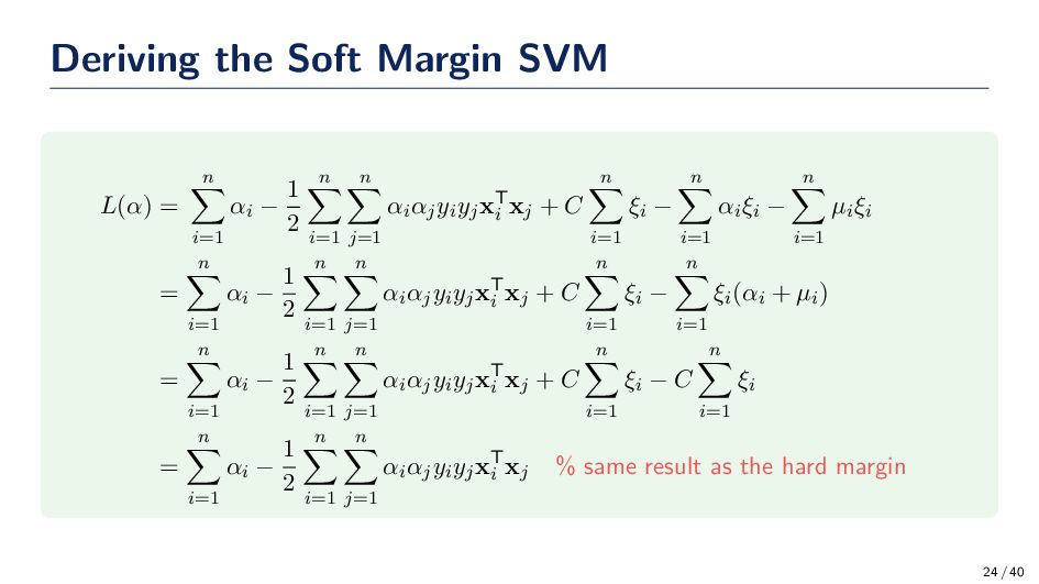
24. Deriving the Soft Margin SVM L(α) = n i=1 αi − 1 2 n i=1 n j=1 αiαjyiyjxT i xj + C n i=1 ξi − n i=1 αiξi − n i=1 µiξi = n i=1 αi − 1 2 n i=1 n j=1 αiαjyiyjxT i xj + C n i=1 ξi − n i=1 ξi(αi + µi) = n i=1 αi − 1 2 n i=1 n j=1 αiαjyiyjxT i xj + C n i=1 ξi − C n i=1 ξi = n i=1 αi − 1 2 n i=1 n j=1 αiαjyiyjxT i xj % same result as the hard margin 24 / 40
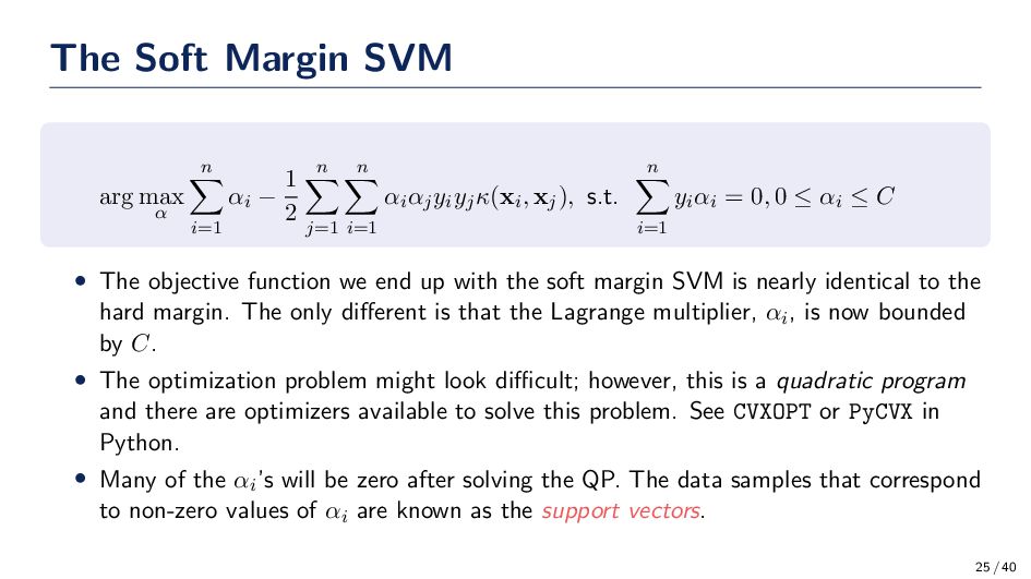
25. The Soft Margin SVM arg max α n i=1 αi − 1 2 n j=1 n i=1 αiαjyiyjκ(xi, xj), s.t. n i=1 yiαi = 0, 0 ≤ αi ≤ C • The objective function we end up with the soft margin SVM is nearly identical to the hard margin. The only different is that the Lagrange multiplier, αi, is now bounded by C. • The optimization problem might look difficult; however, this is a quadratic program and there are optimizers available to solve this problem. See CVXOPT or PyCVX in Python. • Many of the αi’s will be zero after solving the QP. The data samples that correspond to non-zero values of αi are known as the support vectors. 25 / 40
26. Sequential Minimal Optimization 26 / 40
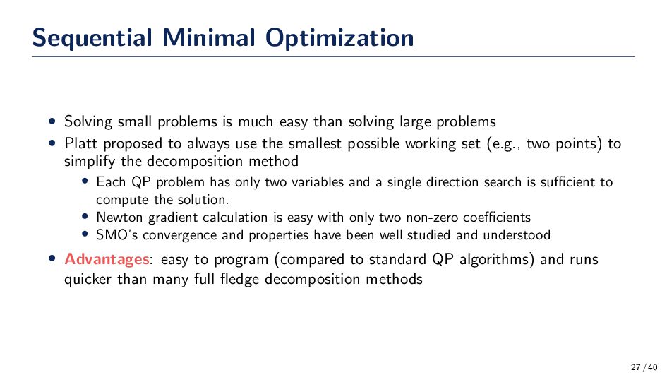
27. Sequential Minimal Optimization • Solving small problems is much easy than solving large problems • Platt proposed to always use the smallest possible working set (e.g., two points) to simplify the decomposition method • Each QP problem has only two variables and a single direction search is sufficient to compute the solution. • Newton gradient calculation is easy with only two non-zero coefficients • SMO’s convergence and properties have been well studied and understood • Advantages: easy to program (compared to standard QP algorithms) and runs quicker than many full fledge decomposition methods 27 / 40
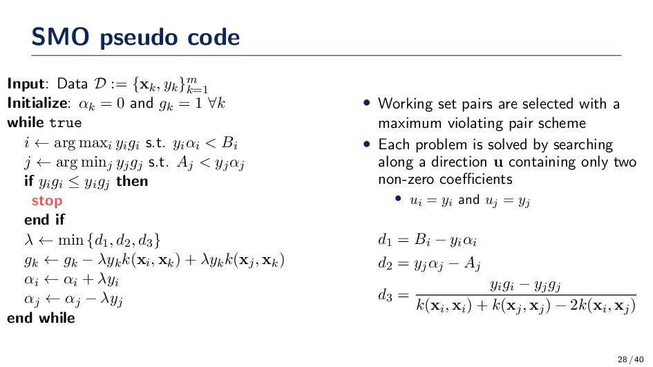
28. SMO pseudo code Input: Data D := {xk, yk}m k=1 Initialize: αk = 0 and gk = 1 ∀k while true i ← arg maxi yigi s.t. yiαi < Bi j ← arg minj yjgj s.t. Aj < yjαj if yigi ≤ yigj then stop end if λ ← min {d1, d2, d3} gk ← gk − λykk(xi, xk) + λykk(xj, xk) αi ← αi + λyi αj ← αj − λyj end while • Working set pairs are selected with a maximum violating pair scheme • Each problem is solved by searching along a direction u containing only two non-zero coefficients • ui = yi and uj = yj d1 = Bi − yiαi d2 = yjαj − Aj d3 = yigi − yjgj k(xi, xi) + k(xj, xj) − 2k(xi, xj) 28 / 40
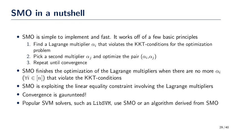
29. SMO in a nutshell • SMO is simple to implement and fast. It works off of a few basic principles 1. Find a Lagrange multiplier αi that violates the KKT-conditions for the optimization problem 2. Pick a second multiplier αj and optimize the pair (αi ,αj ) 3. Repeat until convergence • SMO finishes the optimization of the Lagrange multipliers when there are no more αi (∀i ∈ [n]) that violate the KKT-conditions • SMO is exploiting the linear equality constraint involving the Lagrange multipliers • Convergence is gaurunteed! • Popular SVM solvers, such as LibSVM, use SMO or an algorithm derived from SMO 29 / 40
30. Kernels 30 / 40
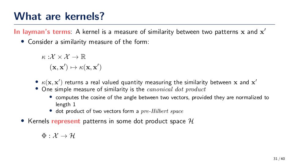
31. What are kernels? In layman’s terms: A kernel is a measure of similarity between two patterns x and x′ • Consider a similarity measure of the form: κ :X × X → R (x, x′) → κ(x, x′) • κ(x, x′) returns a real valued quantity measuring the similarity between x and x′ • One simple measure of similarity is the canonical dot product • computes the cosine of the angle between two vectors, provided they are normalized to length 1 • dot product of two vectors form a pre-Hilbert space • Kernels represent patterns in some dot product space H Φ : X → H 31 / 40
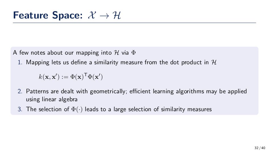
32. Feature Space: X → H A few notes about our mapping into H via Φ 1. Mapping lets us define a similarity measure from the dot product in H k(x, x′) := Φ(x)TΦ(x′) 2. Patterns are dealt with geometrically; efficient learning algorithms may be applied using linear algebra 3. The selection of Φ(·) leads to a large selection of similarity measures 32 / 40
33. A simple kernel example Consider the following dot product:   x2 1 √ 2x1x2 x2 2   T   x2 1 √ 2x1x2 x2 2   = x2 1 x2 1 + 2x2 1 x2 2 + x2 2 x2 2 = (x2 1 + x2 2 )2 = x1 x2 T x1 x2 2 = (xTx)2 Φ(x)TΦ(x) = κ(x, x) Can you think of a kernel where to dot product occurs in an infinite dimensional space? Why? 33 / 40
34. A simple kernel example 4 2 0 2 4 4 2 0 2 4 0 5 10 15 20 25 20 0 20 0 5 10 15 20 25 34 / 40
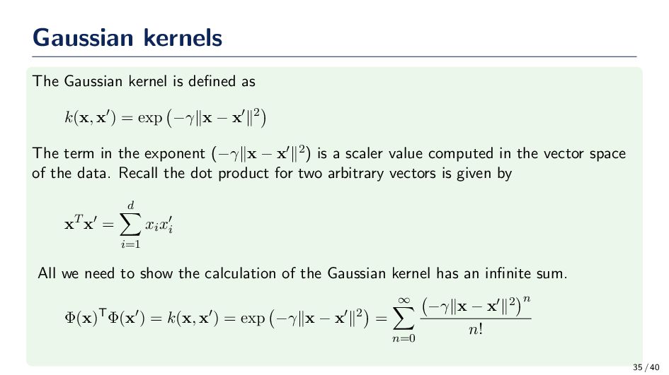
35. Gaussian kernels The Gaussian kernel is defined as k(x, x′) = exp −γ∥x − x′∥2 The term in the exponent (−γ∥x − x′∥2) is a scaler value computed in the vector space of the data. Recall the dot product for two arbitrary vectors is given by xT x′ = d i=1 xix′ i All we need to show the calculation of the Gaussian kernel has an infinite sum. Φ(x)TΦ(x′) = k(x, x′) = exp −γ∥x − x′∥2 = ∞ n=0 −γ∥x − x′∥2 n n! 35 / 40
36. The Kernel Trick • The “trick” in each of the kernel examples is that we never needed to calculate Φ(x). Instead, we applied a nonlinear function to a dot product and this was equivalent to the dot product in a high dimensional space. • This is known as the kernel trick! • Kernels allow us to solve nonlinear classification problems by taking advantage of Cover’s Theorem without the overhead of finding the high dimensional space. 36 / 40
37. Other popular kernel choices Radial Basis Kernel κ(x, z) = exp −γ∥x − z∥2 Polynomial Kernel κ(x, z) = (αxTz + β)p Hyperbolic Tangent Kernel κ(x, z) = tanh(αxTz + β) 37 / 40
38. Summary 38 / 40
39. References Christopher Bishop (2007) Pattern Recognition and Machine Learning New York, NY: Springer 1st edition. Vladimir Vapnik (2000) The Nature of Statistical Learning New York, NY: Springer 1st edition. Christopher Burges (1998) A Tutorial on Support Vector Machines for Pattern Recognition Data Mining and Knowledge Discovery, pp. 121–167. 39 / 40
40. The End 40 / 40