Chapters 3 & 4. Many of the topics discussed today fall under the umbrella of unsupervised learning. That is learning from unlabeled data. Topics • Parametric: maximum likelihood estimator, Bayesian estimation • Non–parametric: kernel density estimation, mixture models, generalized view of EM • Clustering: k–means, expectation maximization About the figures: many of the figures were collected from the Pattern Classification & PRML text, along with some figures generated by custom Matlab and Python scripts. Also, much of the content of the lecture is derived from previous years lectures of this course. 4 / 69
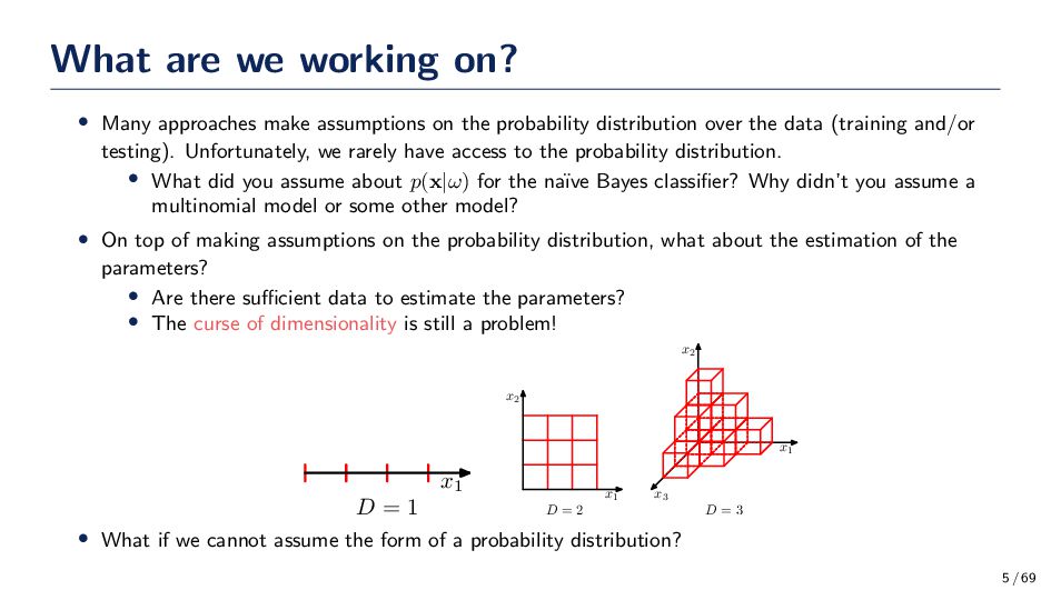
on the probability distribution over the data (training and/or testing). Unfortunately, we rarely have access to the probability distribution. • What did you assume about p(x|ω) for the na¨ ıve Bayes classifier? Why didn’t you assume a multinomial model or some other model? • On top of making assumptions on the probability distribution, what about the estimation of the parameters? • Are there sufficient data to estimate the parameters? • The curse of dimensionality is still a problem! x1 D = 1 x1 x2 D = 2 x1 x2 x3 D = 3 • What if we cannot assume the form of a probability distribution? 5 / 69
the properties and computation of functions such as p(x) that govern the behavior of a probability distribution. For example, if X is distributed as a Gaussian random variable, then the probability distribution for X has parameters µ and σ2. The distribution is of the form, p(X = x) = 1 √ 2πσ e− (x−µ)2 2σ2 • The Bayes classifier required that you know P(ω), p(x|ω), and p(x) • p(x) can be computed using the total probability theorem • What if the distribution on ω and/or the x’s conditional distribution on ω is unknown? • We can assume the form of the distribution, but how do we know if it is correct or approximately correct? • One option is to use the Kolmorogrov-Smirnov test to test against a distribution • How much data are sufficient to estimate the parameters? • If we can (cannot) assume the form of the distribution, we use parametric (nonparametric) techniques 7 / 69
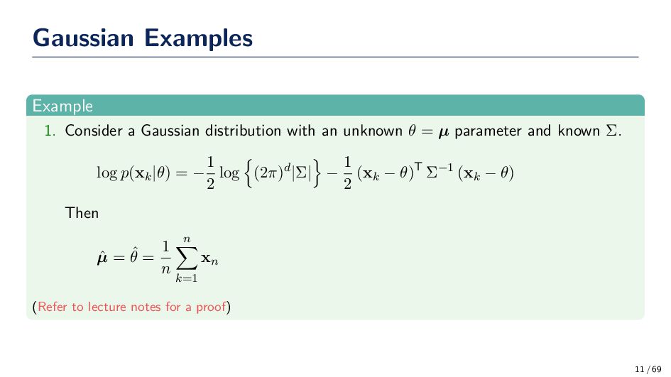
sets Dj for j = {1, . . . , c} (i.e., one for each class – p(x|ωj )). Dj is sampled from a probability distribution with parameters θj (e.g., for a Gaussian distribution θj = {µj , Σj }). Suppose a data set D has n samples drawn iid. The likelihood of the data for a set of parameters is, p(D|θ) = n k=1 p(xk |θ) ⇒ log p(D|θ) = n k=1 log p(xk |θ) • p(D|θ) is the likelihood of D given θ • The maximum-likelihood estimate of θ is given by the ˆ θ that satisfies, ˆ θ = arg max θ∈Θ {p(D|θ)} = arg max θ∈Θ {log p(D|θ)} = arg max θ∈Θ {l(θ)} • ˆ θ best supports the observed data 8 / 69
less work. Finding the MLE, ˆ θ, is found by setting the gradient of l(θ) equal to zero. That is, ∇θ l(θ) = n k=1 ∇θ log p(xk |θ) Solving for ˆ θ A solution to ˆ θ is found by setting the gradient equal to zero ∇θ l(θ) = 0 • The solution to ˆ θ could be a global max, local min or max or (rarely) an inflection point, so you must check. ˆ θ is only an estimate! 9 / 69
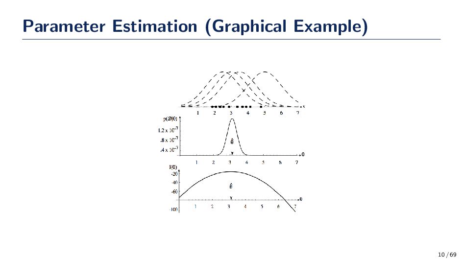
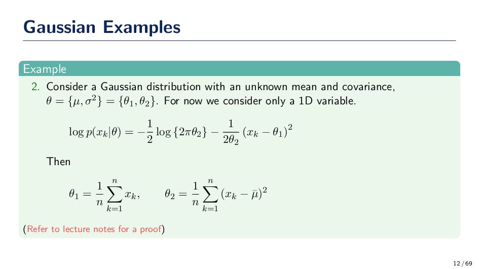
unknown mean and covariance, θ = {µ, σ2} = {θ1 , θ2 }. For now we consider only a 1D variable. log p(xk |θ) = − 1 2 log {2πθ2 } − 1 2θ2 (xk − θ1 )2 Then θ1 = 1 n n k=1 xk , θ2 = 1 n n k=1 (xk − ¯ µ)2 (Refer to lecture notes for a proof) 12 / 69
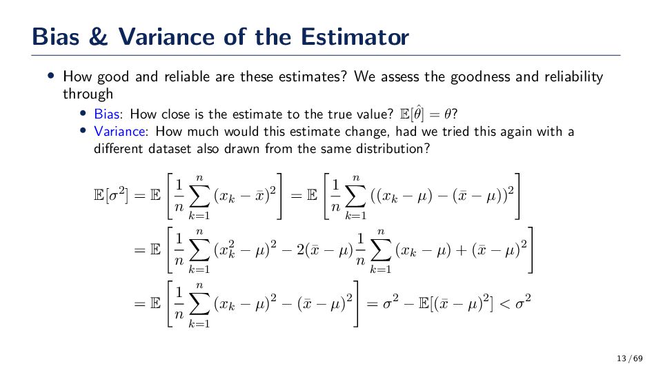
reliable are these estimates? We assess the goodness and reliability through • Bias: How close is the estimate to the true value? E[ˆ θ] = θ? • Variance: How much would this estimate change, had we tried this again with a different dataset also drawn from the same distribution? E[σ2] = E 1 n n k=1 (xk − ¯ x)2 = E 1 n n k=1 ((xk − µ) − (¯ x − µ))2 = E 1 n n k=1 (x2 k − µ)2 − 2(¯ x − µ) 1 n n k=1 (xk − µ) + (¯ x − µ)2 = E 1 n n k=1 (xk − µ)2 − (¯ x − µ)2 = σ2 − E[(¯ x − µ)2] < σ2 13 / 69
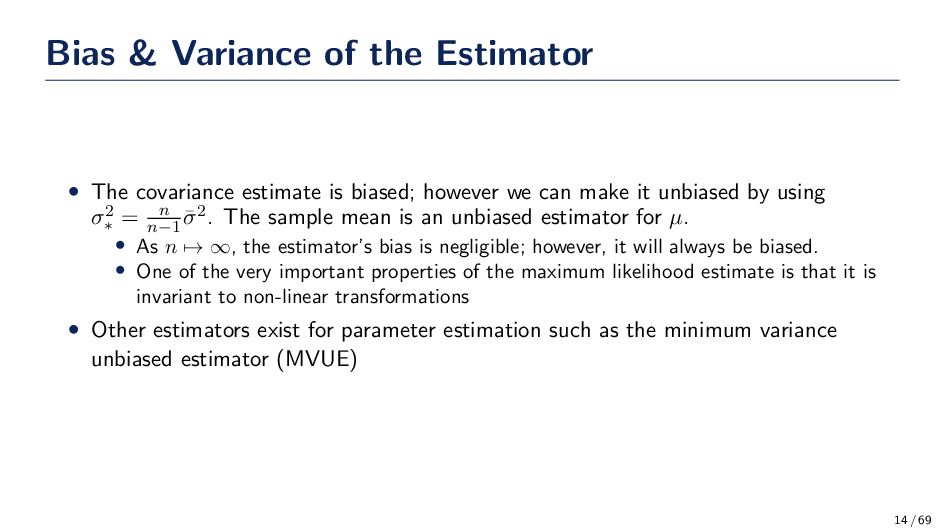
is biased; however we can make it unbiased by using σ2 ∗ = n n−1 ¯ σ2. The sample mean is an unbiased estimator for µ. • As n → ∞, the estimator’s bias is negligible; however, it will always be biased. • One of the very important properties of the maximum likelihood estimate is that it is invariant to non-linear transformations • Other estimators exist for parameter estimation such as the minimum variance unbiased estimator (MVUE) 14 / 69
be fixed, but unknown. Bayesian Estimation (BE) assumes θ are random variables and instead of finding ˆ θ we find p(θ|D). • BE generally provides us with more information; however, computing θBE may be more involved than θMLE. • Bayesian estimation is not estimating θ, rather we are finding the distribution p(x|D) based on the observation of D • For most practical applications, if the assumptions are correct, and there is sufficient data MLE gives good results • MLE: Frequentist approach • BE: Bayesian approach • The MLE method found the estimator that maximized the log-likelihood function, p(D|θ). Why didn’t we use the a priori density p(θ|D)? Such methods that use p(θ|D) are referred to as Bayesian estimation techniques. 15 / 69
of the density p(x|θ) is assumed to be known, but the value of the parameter vector θ is not known exactly. 2. Our initial knowledge about θ is contained in a known a priori density p(θ). 3. The rest of our knowledge about θ is contained in a set D of n samples x1 , . . . , xn drawn independently according to the unknown probability density p(x). According to Bayes theorem and independence of x we have, p(θ|D) = p(θ)p(D|θ) p(θ)p(D|θ)dθ , p(D|θ) = N k=1 p(xk |θ) Suppose that p(D|θ) reaches a sharp peak at θ = ˆ θ. If the prior density p(θ) is not zero at θ = ˆ θ and does not change much in the surrounding neighborhood, then p(θ|D) also peaks at that point. 16 / 69
Mentality Choose the parameters that maximize the likelihood of the data being observed, θMLE = arg max θ∈Θ p(D|θ) The Frequentist (MLE) Mentality Choose the parameters that maximize the posterior probability of θ given the observed data θMAP = arg max θ∈Θ p(θ|D) 17 / 69
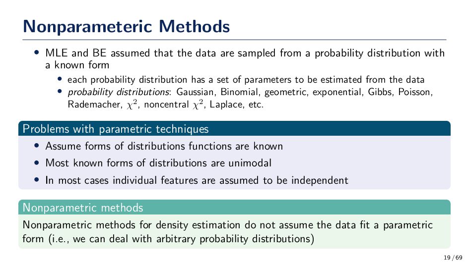
are sampled from a probability distribution with a known form • each probability distribution has a set of parameters to be estimated from the data • probability distributions: Gaussian, Binomial, geometric, exponential, Gibbs, Poisson, Rademacher, χ2, noncentral χ2, Laplace, etc. Problems with parametric techniques • Assume forms of distributions functions are known • Most known forms of distributions are unimodal • In most cases individual features are assumed to be independent Nonparametric methods Nonparametric methods for density estimation do not assume the data fit a parametric form (i.e., we can deal with arbitrary probability distributions) 19 / 69
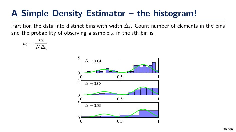
into distinct bins with width ∆i. Count number of elements in the bins and the probability of observing a sample x in the ith bin is, pi = ni N∆i ∆ = 0.04 0 0.5 1 0 5 ∆ = 0.08 0 0.5 1 0 5 ∆ = 0.25 0 0.5 1 0 5 20 / 69
many density estimation methods are very simple. The most fundamental techniques rely on the fact that the probability P that a vector x will fall in a region R is given by P = R p(x′)dx′ • P is a smoothed or averaged version of the density function p(x) • we can estimate this smoothed value of p by estimating the probability P 21 / 69
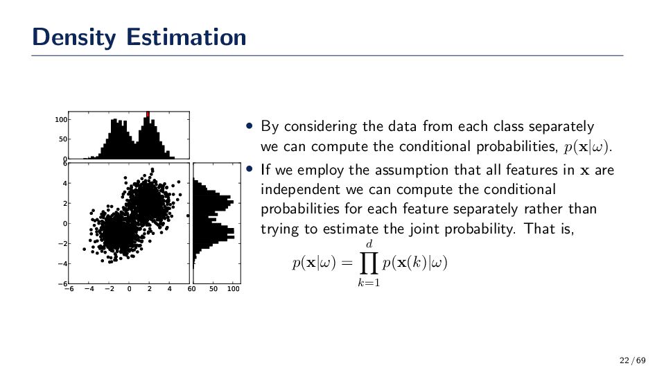
4 2 0 2 4 6 0 50 100 0 50 100 • By considering the data from each class separately we can compute the conditional probabilities, p(x|ω). • If we employ the assumption that all features in x are independent we can compute the conditional probabilities for each feature separately rather than trying to estimate the joint probability. That is, p(x|ω) = d k=1 p(x(k)|ω) 22 / 69
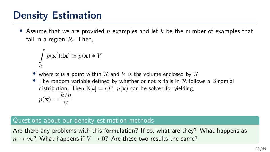
and let k be the number of examples that fall in a region R. Then, R p(x′)dx′ ≃ p(x) ∗ V • where x is a point within R and V is the volume enclosed by R • The random variable defined by whether or not x falls in R follows a Binomial distribution. Then E[k] = nP. p(x) can be solved for yielding, p(x) = k/n V Questions about our density estimation methods Are there any problems with this formulation? If so, what are they? What happens as n → ∞? What happens if V → 0? Are these two results the same? 23 / 69
estimation in one of two ways. First, we could fix V and let n grow to infinity, or fix n and let V approach zero. Lets examine what happens. • If we fix the volume V and take more and more training samples, the ratio k/n will converge (in probability), but we have only obtained an estimate of the space-averaged value of p(x). • If we want to obtain p(x) rather than just an averaged version of it, we must be prepared to let V approach zero. Thus we must fix n and let V approach zero. However, eventually p(x) ≃ 0 since V → 0. Thus, letting V → 0 is a useless result. • Since V → 0 is not an option, we must live with a finite sample estimation of p(x) that will contain some variance in the estimation. How can we choose V ? • It should be large enough to contain plenty of samples in R • It should be small enough to justify the assumption of p(x) be constant within the chosen V / R. 24 / 69
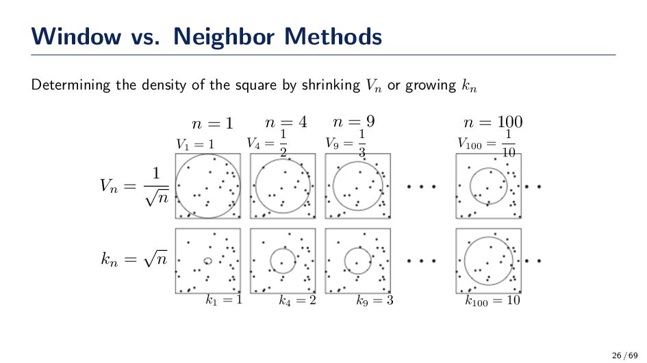
(x) is to converge to p(x), 3 conditions are required: Case 1 This condition assures us that the space averaged P/V will converge to p(x), provided that the regions shrink uniformly. lim n→∞ Vn = 0 Case 2 This condition, which only makes sense if p(x) ̸= 0, assures us that the frequency ratio will converge (in probability) to the probability P. lim n→∞ kn = ∞ Case 3 This condition is clearly necessary if pn (x) is to converge at all. lim n→∞ kn n = 0 • There are two common ways of obtaining sequences of regions that satisfy these conditions 1. Shrink an initial region by specifying the volume Vn as some function of n (Parzen Window) 2. Specify kn as some function of n (Nearest Neighbor) 25 / 69
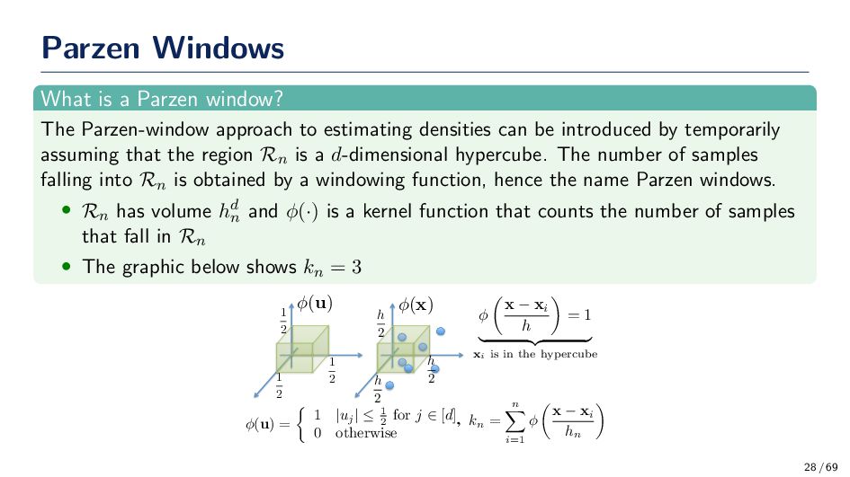
to estimating densities can be introduced by temporarily assuming that the region Rn is a d-dimensional hypercube. The number of samples falling into Rn is obtained by a windowing function, hence the name Parzen windows. • Rn has volume hd n and ϕ(·) is a kernel function that counts the number of samples that fall in Rn • The graphic below shows kn = 3 (u) = ⇢ 1 |uj | 1 2 for j 2 [d] 0 otherwise (u) 1 2 1 2 1 2 (x) h 2 h 2 h 2 ✓ x xi h ◆ = 1 | {z } xi is in the hypercube kn = n X i=1 ✓ x xi hn ◆ , 28 / 69
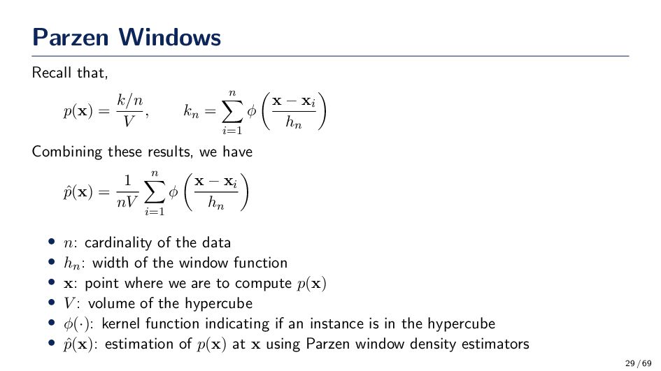
= n i=1 ϕ x − xi hn Combining these results, we have ˆ p(x) = 1 nV n i=1 ϕ x − xi hn • n: cardinality of the data • hn: width of the window function • x: point where we are to compute p(x) • V : volume of the hypercube • ϕ(·): kernel function indicating if an instance is in the hypercube • ˆ p(x): estimation of p(x) at x using Parzen window density estimators 29 / 69
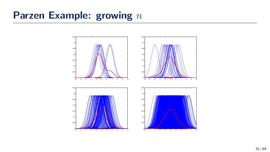
the density estimator ˆ p(x) = 1 nhd n n i=1 ϕ x − xi hn • Consider ϕ(·) as a general smoothing function, such that ϕ(x) ≥ 0 (nonnegativity), and ϕ(x)dx = 1 (normalization). The general expression for ˆ p(x) remains unchanged with these constraints. • ˆ p(x) can be viewed as a superposition of the ϕ(·)’s, which is a measurement of how far x is from xi, around the point x which we are trying to estimate. • xi ’s are the training data in D and ˆ p(x) is an interpolation of the contribution of each sample. The kernel determines the value of xi ’s “relatedness” to x. • Given the constraints above ϕ is a distribution function, ˆ p(x) converges in probability with n → ∞. 30 / 69
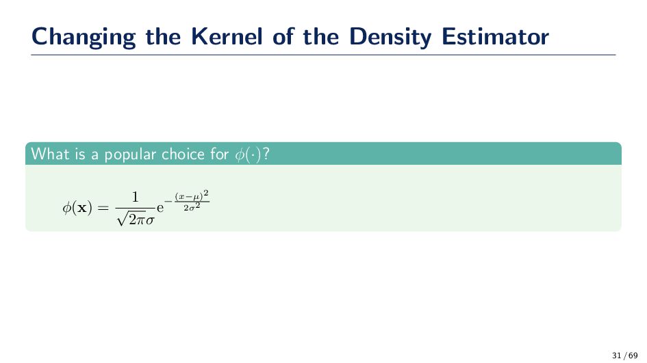
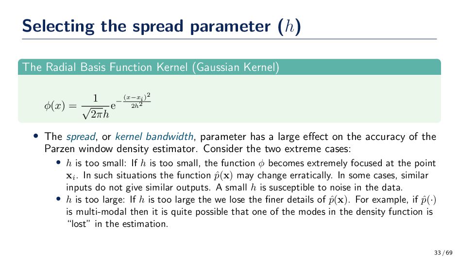
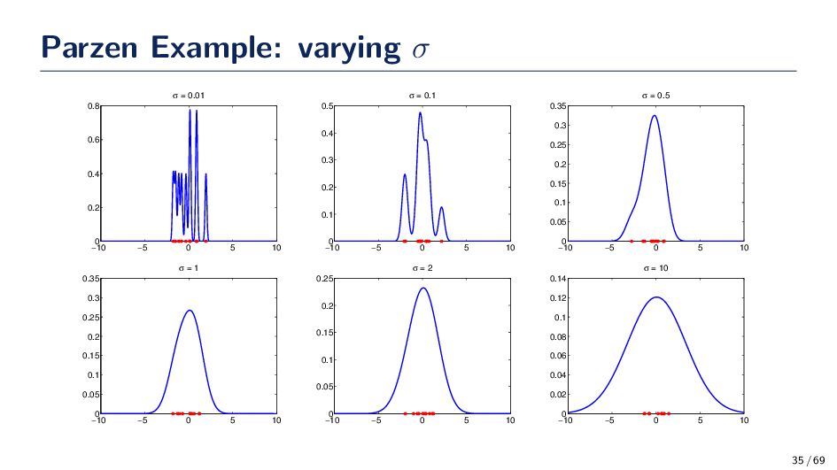
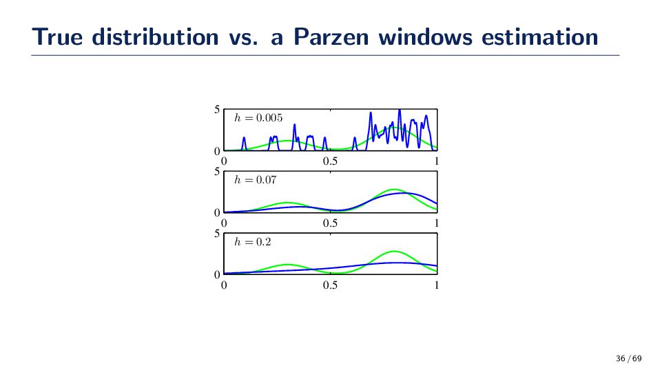
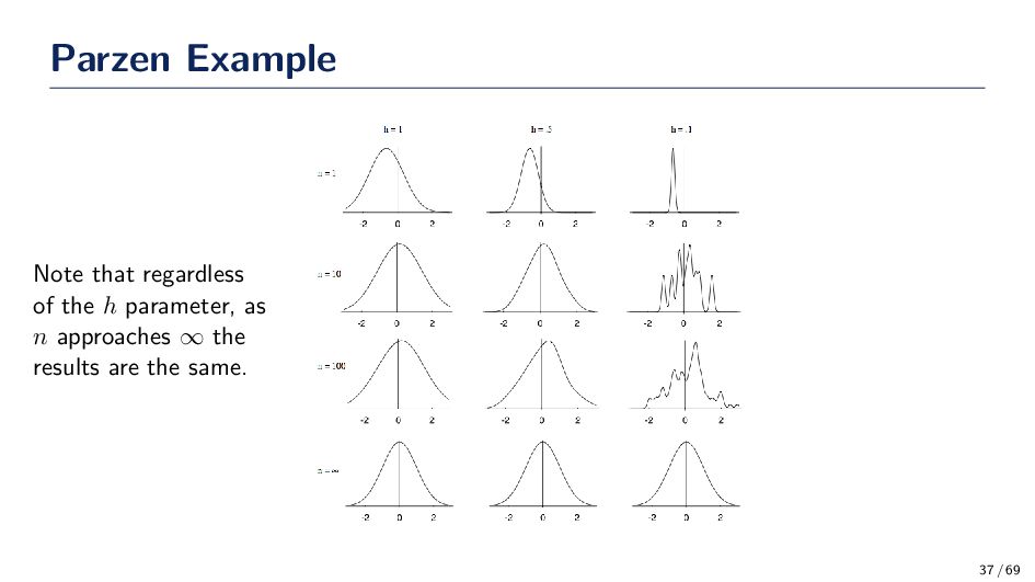
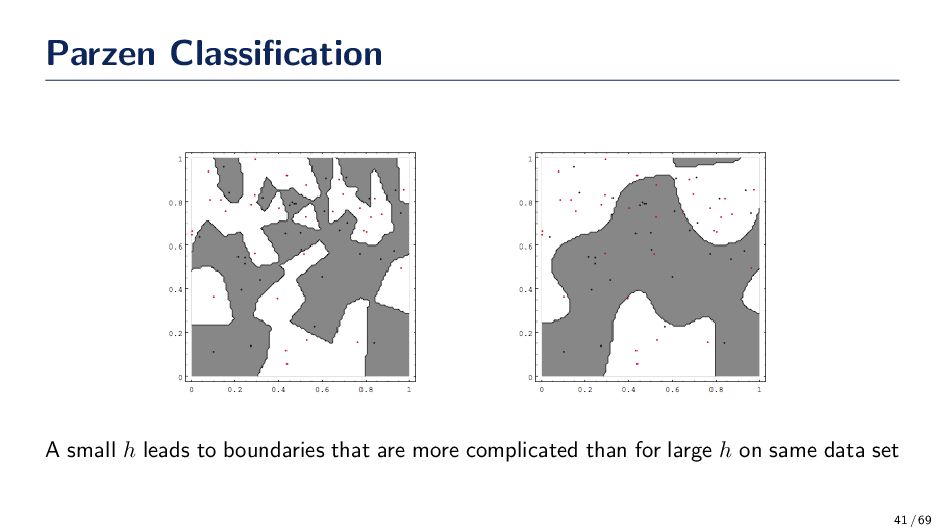
(Gaussian Kernel) ϕ(x) = 1 √ 2πh e−(x−xi)2 2h2 • The spread, or kernel bandwidth, parameter has a large effect on the accuracy of the Parzen window density estimator. Consider the two extreme cases: • h is too small: If h is too small, the function ϕ becomes extremely focused at the point xi. In such situations the function ˆ p(x) may change erratically. In some cases, similar inputs do not give similar outputs. A small h is susceptible to noise in the data. • h is too large: If h is too large the we lose the finer details of ˆ p(x). For example, if ˆ p(·) is multi-modal then it is quite possible that one of the modes in the density function is “lost” in the estimation. 33 / 69
1D kernels (product kernels). ˆ pp (x) = 1 n n i=1 ϕ(x, xi , h1 , . . . , hd ) where ϕ(x, xi , h1 , . . . , hd ) = 1 h1 h2 · · · hd d j=1 ϕj x(j) − xi (j) hj Kernel Independence Kernel independence is assumed above – which does NOT imply feature independence, ˆ pp (x) = d j=1 1 nhj n i=1 ϕj x(j) − xi (j) hj 38 / 69
rule is implemented as follows, ω∗ = arg max ω∈Ω p(x|ω)P(ω) p(x) = arg max ω∈Ω p(x|ω)P(ω) • Use the data in D to estimate p(x|ω) for ω ∈ Ω using the Parzen window density estimator. Define a Bernoulli random variable zi,c that takes value 1 if xi belongs to ωc and 0 if it does not. The MLE for the prior probabilities (yes, you can use the MLE on probabilities – see DHS Ch. 2, exercise 3) is given by, P(ωc ) = 1 n n i=1 zi,c. 39 / 69
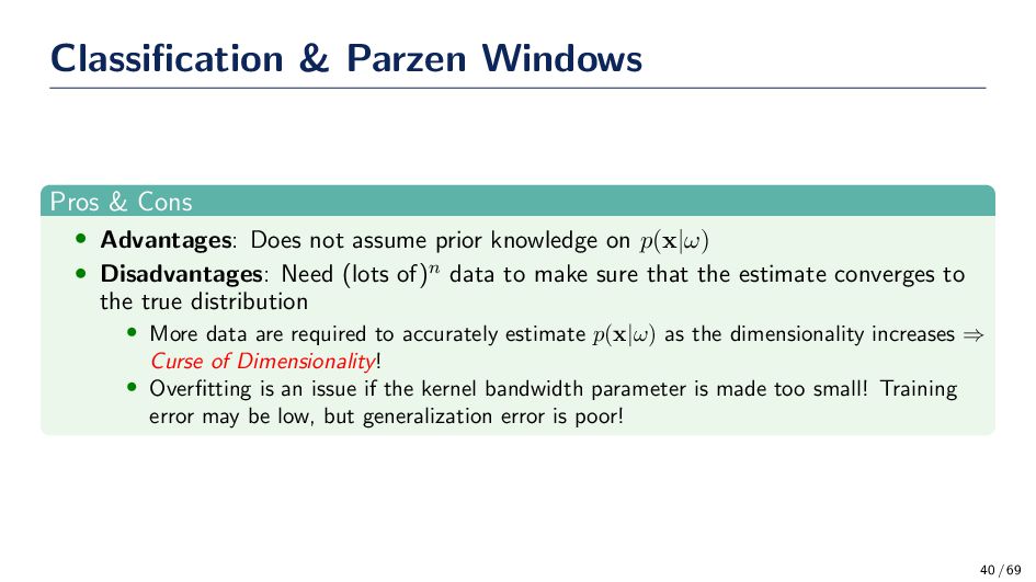
not assume prior knowledge on p(x|ω) • Disadvantages: Need (lots of)n data to make sure that the estimate converges to the true distribution • More data are required to accurately estimate p(x|ω) as the dimensionality increases ⇒ Curse of Dimensionality! • Overfitting is an issue if the kernel bandwidth parameter is made too small! Training error may be low, but generalization error is poor! 40 / 69
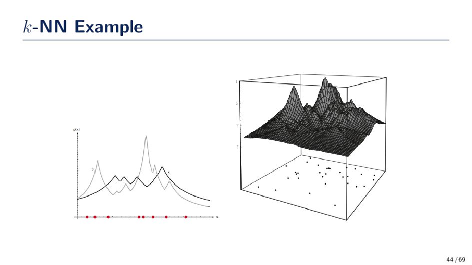
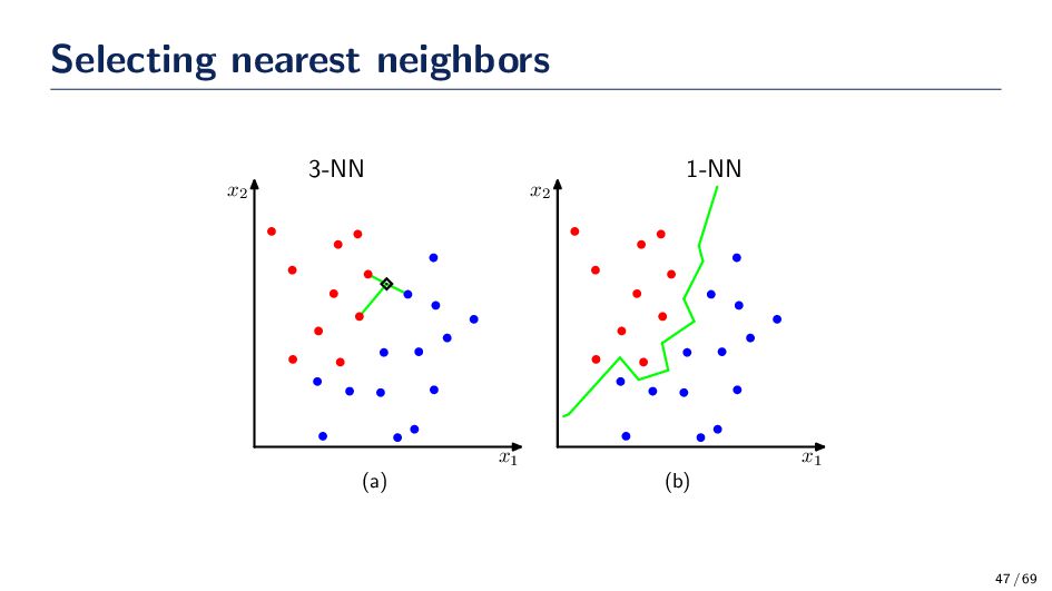
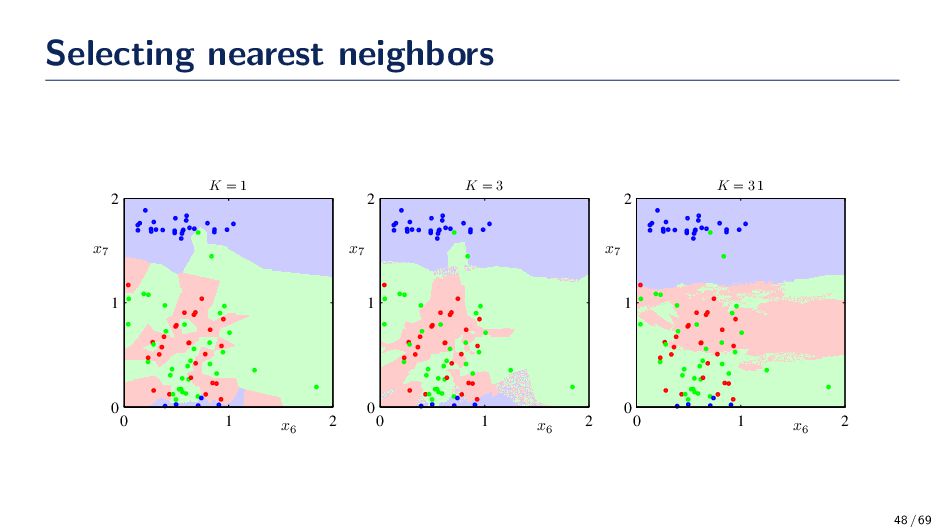
to use and what should the parameters of the function be set to (e.g., σ, h) • A remedy to this problem is to let the volume be a function of the training data. That is fix the value of the k-nearest neighbors and determine the minimum volume that encloses the k samples. • If the density near x is high them volume will be small (small value for the kernel), and if the density near x is low, the volume will be large (large value for the kernel). Thus, k-NN is “automatically” determining the window size for the training data. k-Nearest Neighbor Estimation Algorithm 1. Select an initial volume around x to estimate p(x). 2. Grow the window until k samples fall in the region R. The samples in R are the nearest neighbors of x. 3. Estimate the density based on: ˆ p(x) = k/n V 43 / 69
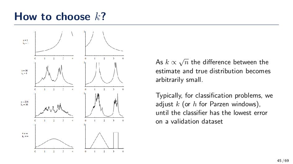
difference between the estimate and true distribution becomes arbitrarily small. Typically, for classification problems, we adjust k (or h for Parzen windows), until the classifier has the lowest error on a validation dataset 45 / 69
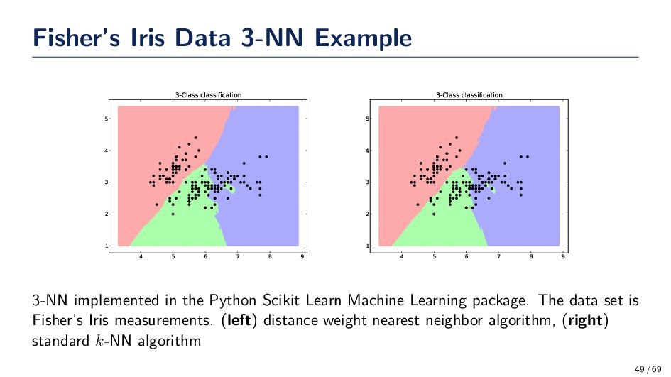
max ωi∈Ω p(x, ωi ) c j=1 p(x, ωj ) • The joint probability, p(x, ωi ), is estimated by placing a volume, V , around point x until k samples fall in the region. Of the k samples ki of them belong to class ωi. The obvious estimate for the joint probability is, pn (x, ωi ) = ki /n V , P(ωi |x) = p(x, ωi ) c j=1 p(x, ωj ) = ki k On your own: Derive the MLE for P(ωi ) and the k-nearest neighbors estimate of p(x) & p(x|ωi ) to show that P(ωi |x) = ki /k. 46 / 69
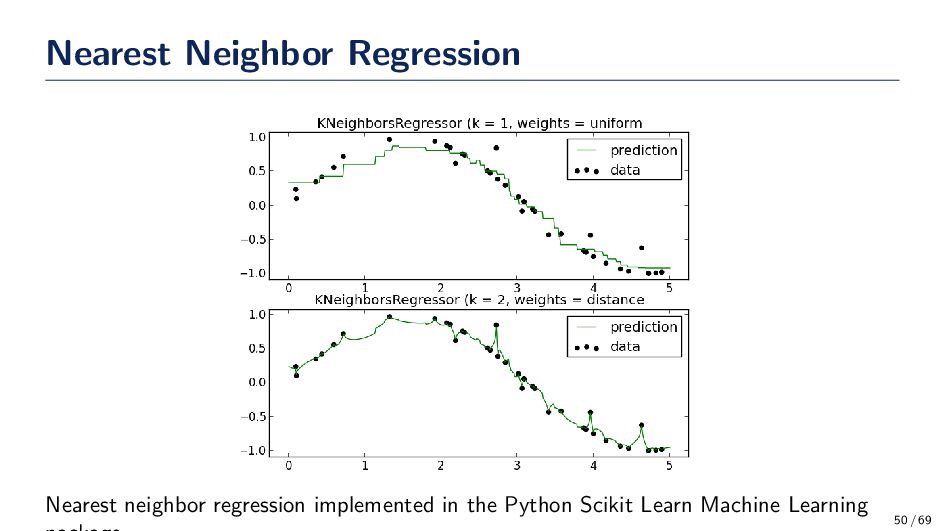
known as a lazy learning because there is no “learning” implemented after the training data set. There are no processing steps required before making a prediction other than receiving the training data. • Since there is no learning implemented in the k-NN and it is based solely on the training data, k-NN is also called memory based learning, or instance based learning. • Computational cost arises from the testing phase and algorithms require larger memory requirements. 51 / 69
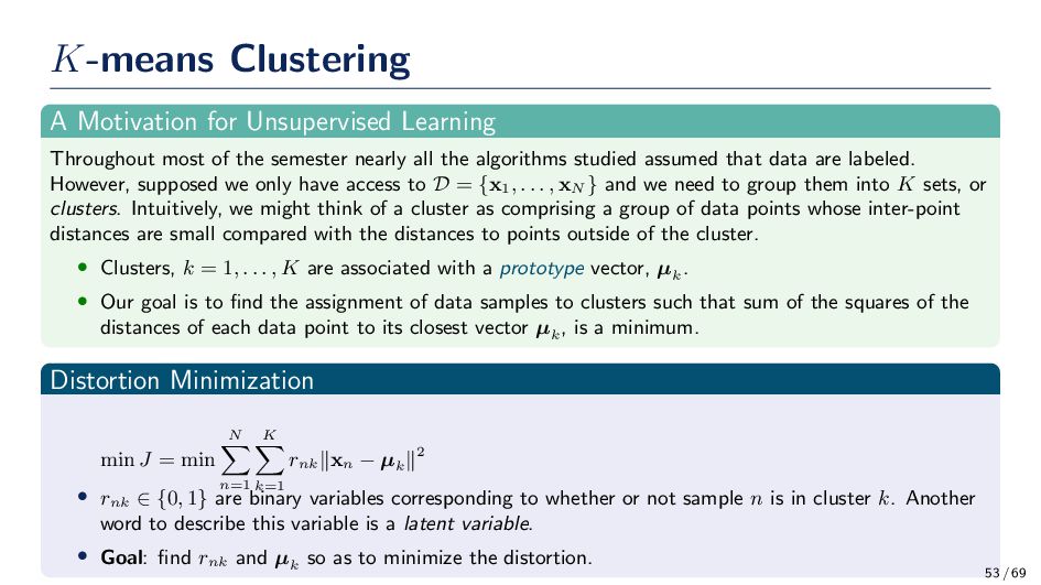
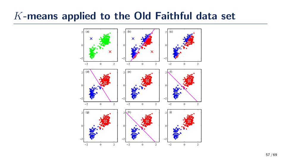
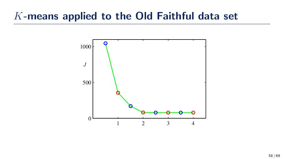
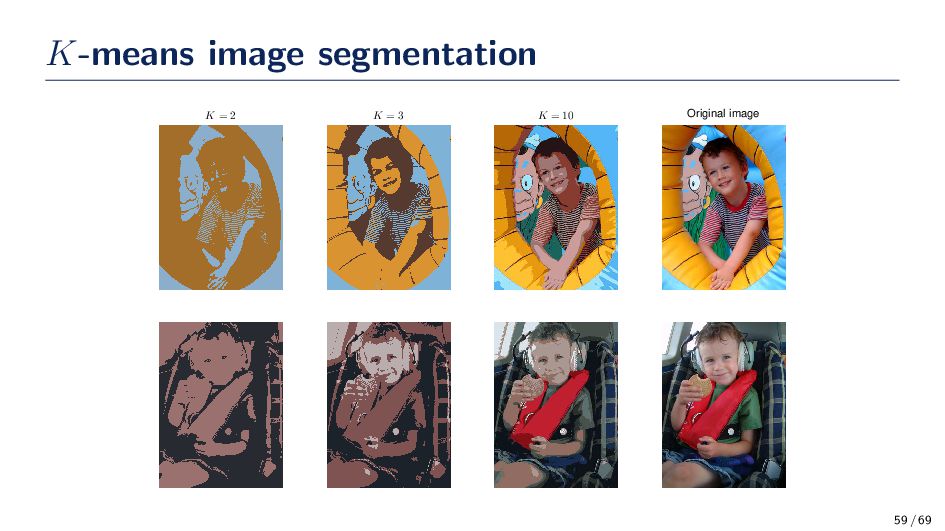
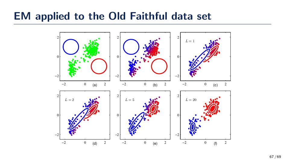
the semester nearly all the algorithms studied assumed that data are labeled. However, supposed we only have access to D = {x1 , . . . , xN } and we need to group them into K sets, or clusters. Intuitively, we might think of a cluster as comprising a group of data points whose inter-point distances are small compared with the distances to points outside of the cluster. • Clusters, k = 1, . . . , K are associated with a prototype vector, µk . • Our goal is to find the assignment of data samples to clusters such that sum of the squares of the distances of each data point to its closest vector µk , is a minimum. Distortion Minimization min J = min N n=1 K k=1 rnk ∥xn − µk ∥2 • rnk ∈ {0, 1} are binary variables corresponding to whether or not sample n is in cluster k. Another word to describe this variable is a latent variable. • Goal: find rnk and µk so as to minimize the distortion. 53 / 69
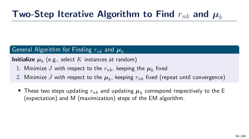
for Finding rnk and µk Initialize µk (e.g., select K instances at random) 1. Minimize J with respect to the rnk, keeping the µk fixed 2. Minimize J with respect to the µk , keeping rnk fixed (repeat until convergence) • These two steps updating rnk and updating µk correspond respectively to the E (expectation) and M (maximization) steps of the EM algorithm. 54 / 69
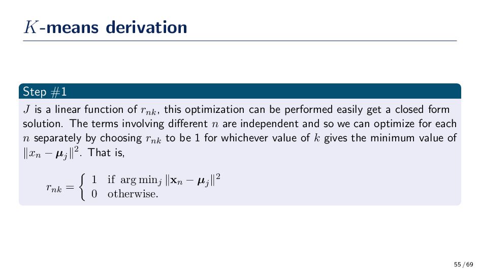
rnk, this optimization can be performed easily get a closed form solution. The terms involving different n are independent and so we can optimize for each n separately by choosing rnk to be 1 for whichever value of k gives the minimum value of ∥xn − µj ∥2. That is, rnk = 1 if arg minj ∥xn − µj ∥2 0 otherwise. 55 / 69
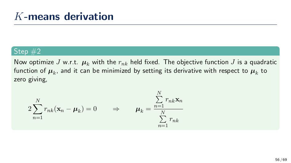
the rnk held fixed. The objective function J is a quadratic function of µk , and it can be minimized by setting its derivative with respect to µk to zero giving, 2 N n=1 rnk (xn − µk ) = 0 ⇒ µk = N n=1 rnk xn N n=1 rnk 56 / 69
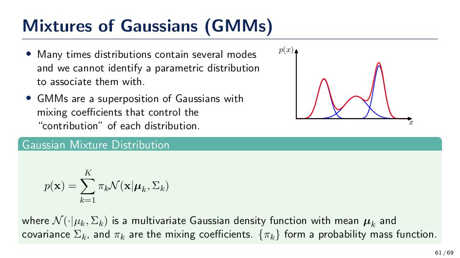
modes and we cannot identify a parametric distribution to associate them with. • GMMs are a superposition of Gaussians with mixing coefficients that control the “contribution” of each distribution. x p(x) Gaussian Mixture Distribution p(x) = K k=1 πk N(x|µk , Σk ) where N(·|µk , Σk ) is a multivariate Gaussian density function with mean µk and covariance Σk, and πk are the mixing coefficients. {πk } form a probability mass function. 61 / 69
∈ {0, 1}K , which a particular element zk is equal to 1 and all other elements equal to 0. There are K possible outcomes for this binary vector. Let πk = p(zk = 1) (i.e., the mixing coefficient), and recall that πk is a pmf (i.e., πk ∈ [0, 1] and πk = 1). The probability of z is, p(z) = p(z1 , . . . , zk ) = K k=1 πzk k Similarly, the conditional distribution of x given a particular value for z is a Gaussian – p(x|zk = 1) = N(x|µk , Σk ). Then, p(x|z) = p(x|z1 , . . . , zk ) = K k=1 N(x|µk , Σk )zk Marginalizing p(x) yeilds p(x) = z∈Z p(x|z)p(z) = K k=1 πk N(x|µk , Σk ) Well isn’t that interesting! The marginal on x can be determined using a set of latent variables. Generally it is easier to work with p(x, z) over p(x). 62 / 69
important role is the conditional probability of z given x. We shall use γ(zk ) to denote p(zk = 1|x), whose value can be found using Bayes’ theorem, γ(zk ) ≡ p(zk = 1|x) = p(zk = 1)p(x|zk = 1) p(x) = πk N(x|µk , Σk ) K k=1 πk N(x|µj , Σj ) • γ(zk ) is a measurement of the responsibility that mixture k claims for the observation x. Why did we just introduce this confusing notation? The latent variables will make our lives easier; however, at the moment life does not seem any easier. Next, let maximize the log-likelihood function for a data set. log p(D|{πk }, {µk }, {Σk }) = N n=1 log K k=1 πk N(xn |µk , Σk ) 63 / 69
with respect to µk and setting the derivative equal to zero yields, 0 = − N n=1 πk N(xn |µk , Σk ) K j=1 πj N(xn |µj , Σj ) γ(znk) Σk (xn − µk ) Assumption Σ−1 k is nonsingular! (Work this out own your own, or ask me after class for a full derivation) Solving for µk µk = 1 Nk N n=1 γ(znk )xn , Nk = N n=1 γ(znk ) 64 / 69
log-likelihood function w.r.t. Σk and πk. Maximizing w.r.t. Σk is straight forward; however, we must be careful with the maximization w.r.t. πk because the solution set is constrained. We must use Lagrange multipliers to find the solution. After all this we find that, Σk = 1 Nk N n=1 γ(znk ) (xn − µk ) (xn − µk )T and πk = Nk N 65 / 69
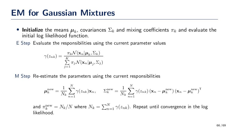
covariances Σk and mixing coefficients πk and evaluate the initial log likelihood function. E Step Evaluate the responsibilities using the current parameter values γ(znk ) = πk N(xn |µk , Σk ) K j=1 πj N(xn |µj , Σj ) M Step Re-estimate the parameters using the current responsibilities µnew k = 1 Nk N n=1 γ(znk )xn , Σnew k = 1 Nk N n=1 γ(znk ) (xn − µnew k ) (xn − µnew k )T and πnew k = Nk /N where Nk = N n=1 γ(znk ). Repeat until convergence in the log likelihood. 66 / 69
![Machine Learning Lectures Density Estimation Gregory Ditzler [email protected] February 24,](https://files.speakerdeck.com/presentations/eeb2b258f42841128f799a6cea4efd82/slide_0.jpg)