Machine Learning Lectures - Dimensionality Reduction

Transcript

1. Machine Learning Lectures Dimensionality Reduction Gregory Ditzler gregory.ditzler@gmail.com February 24, 2024 1 / 48
2. Overview 1. Motivation 2. Principal Component Analysis 3. Multi-Dimensional Scaling 4. Feature Selection 2 / 48
3. Motivation 3 / 48
4. Lecture Overview • There is a curse of dimensionality! The complexity of a model increases with the dimensionality. Sometimes exponentially! • So, why should we perform dimensionality reduction? • reduces the time complexity: less computation • reduces the space complexity: fewer parameters • saves costs: some features/variables cost money • makes interpreting complex high-dimensional data • Can you visualize data with more than 3-dimensions? 4 / 48
5. Principal Component Analysis 5 / 48
6. Principal Components Analysis (PCA) • Principal Components Analysis is an unsupervised dimensionality reduction technique • Dimensionality of data may be large and many algorithms suffer from the curse of dimensionality • Principal components maximize the variance (we will prove this!) • Quite possibly the most popular dimensionality reduction method • Mathematical tools needed: Eigenvalue problem, Lagrange multipliers, and a little bit about moments and variance. ⊗ ⊗ ⊗ ⊗ ⊗ ⊗ ⊗ ⊗ ⊗ ⊗ ⊗ ⊗ ⊗ ⊗ ⊗ ⊗ ⊗ ⊗ ⊗ ⊗ ⊗ ⊗ ⊗ ⊗ ⊗ ⊗ ⊗ ⊗ ⊗ ⊗ ⊗ ⊗ ⊗ ⊗ ⊗ ⊗ ⊗ ⊗ ⊗ ⊗ ⊗ ⊗ ⊗ ⊗ ⊗ ⊗ ⊗ ⊗ ⊗ ⊗ ⊗ e 1 2 3 4 5 6 7 8 9 10 −1 −2 −3 −4 −5 −6 −7 −8 −9 −10 1 2 3 4 5 6 7 8 9 10 −1 −2 −3 −4 −5 −6 −7 −8 −9 −10 ⊗ ⊗ ⊗ ⊗ ⊗ ⊗ ⊗ ⊗ ⊗ ⊗ ⊗ ⊗ ⊗ ⊗ ⊗ ⊗ ⊗ ⊗ ⊗ ⊗ ⊗ ⊗ ⊗ ⊗ ⊗ ⊗ ⊗ ⊗ ⊗ ⊗ ⊗ ⊗ ⊗ ⊗ ⊗ ⊗ ⊗ ⊗ ⊗ ⊗ ⊗ ⊗ ⊗ ⊗ ⊗ ⊗ ⊗ ⊗ ⊗ ⊗ ⊗ ⊗ ⊗ ⊗ ⊗ ⊗ ⊗ ⊗ ⊗ ⊗ ⊗ ⊗ ⊗ ⊗ ⊗ ⊗ ⊗ ⊗ ⊗ ⊗ ⊗ ⊗ ⊗ ⊗ ⊗ ⊗ ⊗ ⊗ ⊗ ⊗ ⊗ ⊗ ⊗ ⊗ ⊗ ⊗ ⊗ ⊗ ⊗ ⊗ ⊗ ⊗ ⊗ ⊗ ⊗ ⊗ ⊗ ⊗ ⊗ ⊗ ⊗ ⊗ ⊗ ⊗ ⊗ ⊗ ⊗ ⊗ ⊗ ⊗ ⊗ ⊗ ⊗ ⊗ ⊗ ⊗ ⊗ ⊗ ⊗ ⊗ ⊗ ⊗ ⊗ ⊗ ⊗ ⊗ ⊗ ⊗ ⊗ ⊗ ⊗ ⊗ ⊗ ⊗ ⊗ e =? 6 / 48
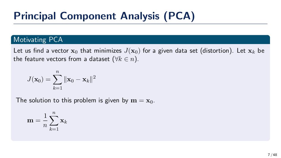
7. Principal Component Analysis (PCA) Motivating PCA Let us find a vector x0 that minimizes J(x0 ) for a given data set (distortion). Let xk be the feature vectors from a dataset (∀k ∈ n). J(x0 ) = n k=1 ∥x0 − xk ∥2 The solution to this problem is given by m = x0. m = 1 n n k=1 xk 7 / 48
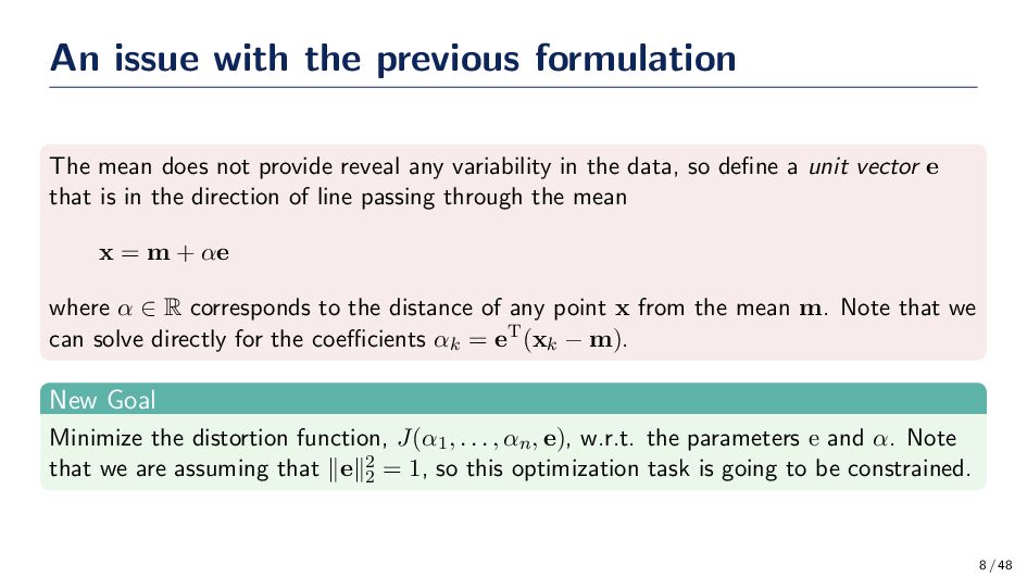
8. An issue with the previous formulation The mean does not provide reveal any variability in the data, so define a unit vector e that is in the direction of line passing through the mean x = m + αe where α ∈ R corresponds to the distance of any point x from the mean m. Note that we can solve directly for the coefficients αk = eT(xk − m). New Goal Minimize the distortion function, J(α1 , . . . , αn , e), w.r.t. the parameters e and α. Note that we are assuming that ∥e∥2 2 = 1, so this optimization task is going to be constrained. 8 / 48
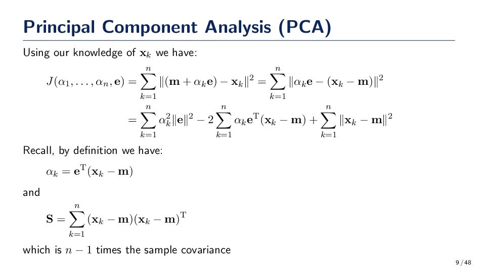
9. Principal Component Analysis (PCA) Using our knowledge of xk we have: J(α1 , . . . , αn , e) = n k=1 ∥(m + αk e) − xk ∥2 = n k=1 ∥αk e − (xk − m)∥2 = n k=1 α2 k ∥e∥2 − 2 n k=1 αk eT(xk − m) + n k=1 ∥xk − m∥2 Recall, by definition we have: αk = eT(xk − m) and S = n k=1 (xk − m)(xk − m)T which is n − 1 times the sample covariance 9 / 48
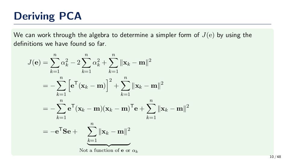
10. Deriving PCA We can work through the algebra to determine a simpler form of J(e) by using the definitions we have found so far. J(e) = n k=1 α2 k − 2 n k=1 α2 k + n k=1 ∥xk − m∥2 = − n k=1 eT(xk − m) 2 + n k=1 ∥xk − m∥2 = − n k=1 eT(xk − m)(xk − m)Te + n k=1 ∥xk − m∥2 = −eTSe + n k=1 ∥xk − m∥2 Not a function of e or αk 10 / 48
11. Deriving PCA • The objective function J(α1 , . . . , αn , e) can be written entirely as a function of e (i.e., J(e)). This appears to be a very convenient solution so far. • This new objective function cannot be optimized directly using standard calculus (e.g., take the derivative and set it equal to zero), because this is a constrained optimization task (i.e., ∥e∥2 2 = 1). 11 / 48
12. 12 / 48
13. 13 / 48
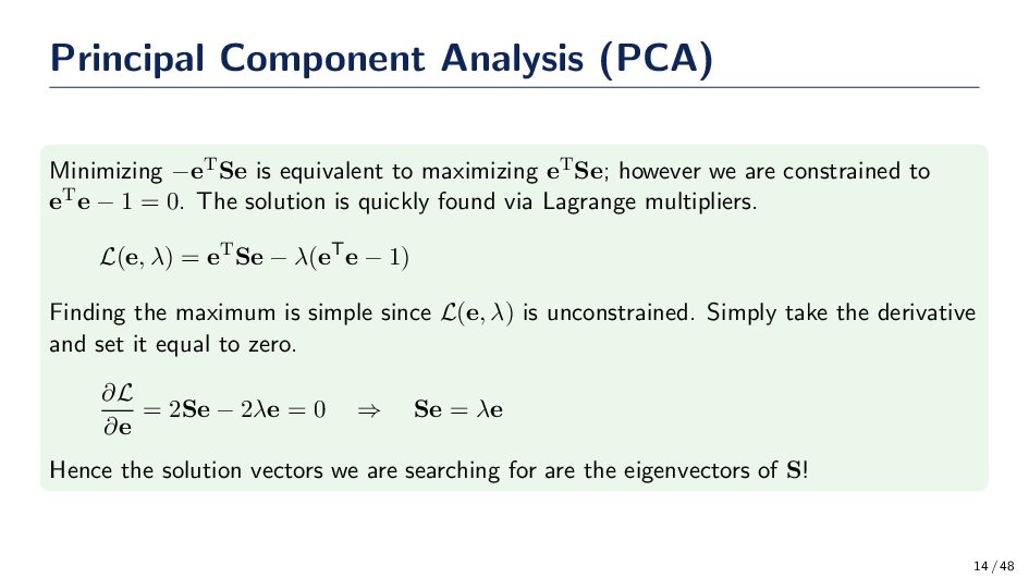
14. Principal Component Analysis (PCA) Minimizing −eTSe is equivalent to maximizing eTSe; however we are constrained to eTe − 1 = 0. The solution is quickly found via Lagrange multipliers. L(e, λ) = eTSe − λ(eTe − 1) Finding the maximum is simple since L(e, λ) is unconstrained. Simply take the derivative and set it equal to zero. ∂L ∂e = 2Se − 2λe = 0 ⇒ Se = λe Hence the solution vectors we are searching for are the eigenvectors of S! 14 / 48
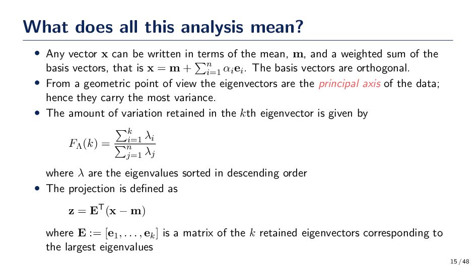
15. What does all this analysis mean? • Any vector x can be written in terms of the mean, m, and a weighted sum of the basis vectors, that is x = m + n i=1 αi ei. The basis vectors are orthogonal. • From a geometric point of view the eigenvectors are the principal axis of the data; hence they carry the most variance. • The amount of variation retained in the kth eigenvector is given by FΛ (k) = k i=1 λi n j=1 λj where λ are the eigenvalues sorted in descending order • The projection is defined as z = ET(x − m) where E := [e1 , . . . , ek ] is a matrix of the k retained eigenvectors corresponding to the largest eigenvalues 15 / 48
16. PCA Applied to Fisher’s Iris Dataset 3 2 1 0 1 2 3 4 PC1 1.0 0.5 0.0 0.5 1.0 1.5 PC2 setosa versicolor virginica 16 / 48
17. PCA Applied to UCI Wine Dataset 4 2 0 2 4 PC1 3 2 1 0 1 2 3 4 PC2 Wine0 Wine1 Wine2 17 / 48
18. PCA Applied to UCI Wine Dataset (No preproc) 400 200 0 200 400 600 800 1000 PC1 20 0 20 40 60 PC2 Wine0 Wine1 Wine2 18 / 48
19. PCA Applied to UCI Wine Dataset 0 2 4 6 8 10 12 PC 6 8 10 12 Variance Explained 19 / 48
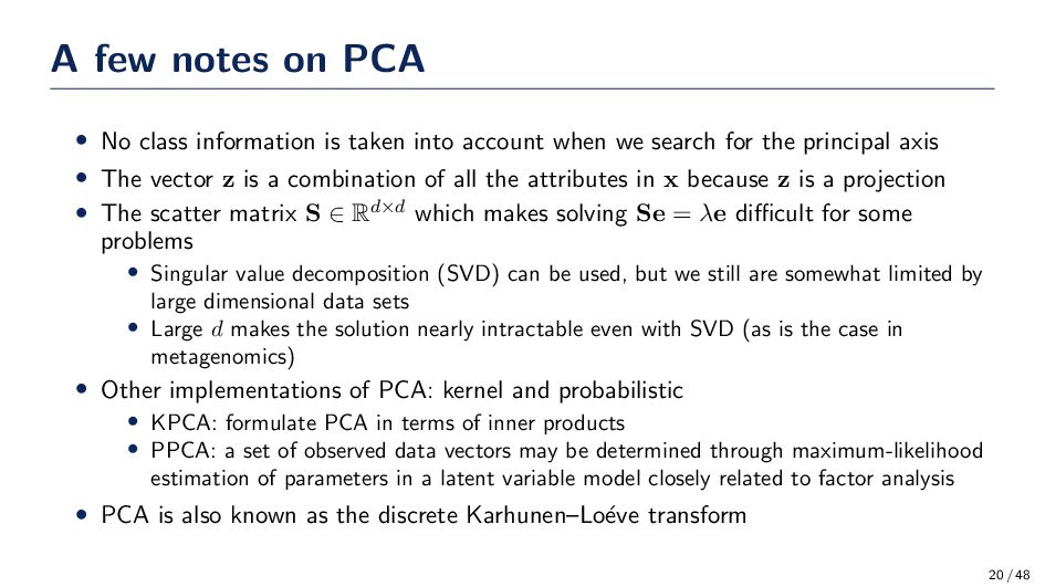
20. A few notes on PCA • No class information is taken into account when we search for the principal axis • The vector z is a combination of all the attributes in x because z is a projection • The scatter matrix S ∈ Rd×d which makes solving Se = λe difficult for some problems • Singular value decomposition (SVD) can be used, but we still are somewhat limited by large dimensional data sets • Large d makes the solution nearly intractable even with SVD (as is the case in metagenomics) • Other implementations of PCA: kernel and probabilistic • KPCA: formulate PCA in terms of inner products • PPCA: a set of observed data vectors may be determined through maximum-likelihood estimation of parameters in a latent variable model closely related to factor analysis • PCA is also known as the discrete Karhunen–Lo´ eve transform 20 / 48
21. Multi-Dimensional Scaling 21 / 48
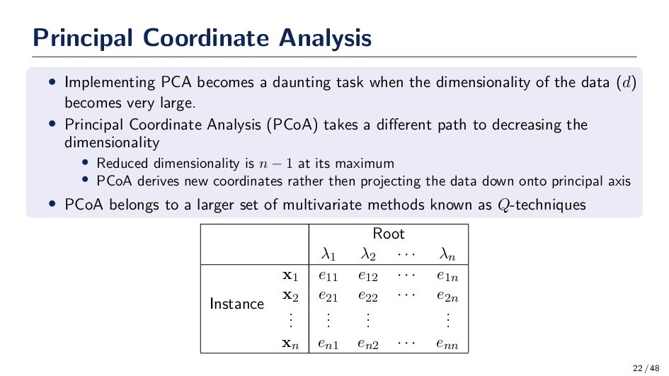
22. Principal Coordinate Analysis • Implementing PCA becomes a daunting task when the dimensionality of the data (d) becomes very large. • Principal Coordinate Analysis (PCoA) takes a different path to decreasing the dimensionality • Reduced dimensionality is n − 1 at its maximum • PCoA derives new coordinates rather then projecting the data down onto principal axis • PCoA belongs to a larger set of multivariate methods known as Q-techniques Root λ1 λ2 · · · λn Instance x1 e11 e12 · · · e1n x2 e21 e22 · · · e2n . . . . . . . . . . . . xn en1 en2 · · · enn 22 / 48
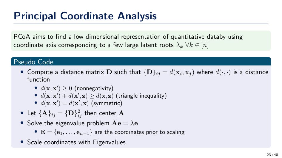
23. Principal Coordinate Analysis PCoA aims to find a low dimensional representation of quantitative databy using coordinate axis corresponding to a few large latent roots λk ∀k ∈ [n] Pseudo Code • Compute a distance matrix D such that {D}ij = d(xi , xj ) where d(·, ·) is a distance function. • d(x, x′) ≥ 0 (nonnegativity) • d(x, x′) + d(x′, z) ≥ d(x, z) (triangle inequality) • d(x, x′) = d(x′, x) (symmetric) • Let {A}ij = {D}2 ij then center A • Solve the eigenvalue problem Ae = λe • E = {e1 , . . . , en−1 } are the coordinates prior to scaling • Scale coordinates with Eigenvalues 23 / 48
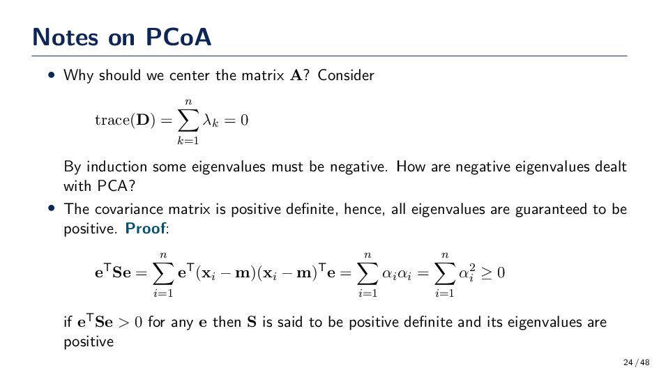
24. Notes on PCoA • Why should we center the matrix A? Consider trace(D) = n k=1 λk = 0 By induction some eigenvalues must be negative. How are negative eigenvalues dealt with PCA? • The covariance matrix is positive definite, hence, all eigenvalues are guaranteed to be positive. Proof: eTSe = n i=1 eT(xi − m)(xi − m)Te = n i=1 αi αi = n i=1 α2 i ≥ 0 if eTSe > 0 for any e then S is said to be positive definite and its eigenvalues are positive 24 / 48
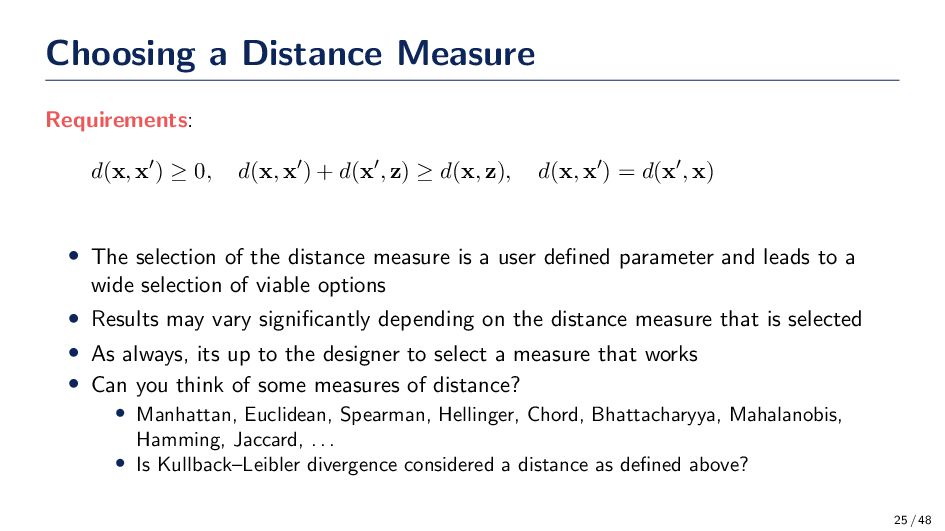
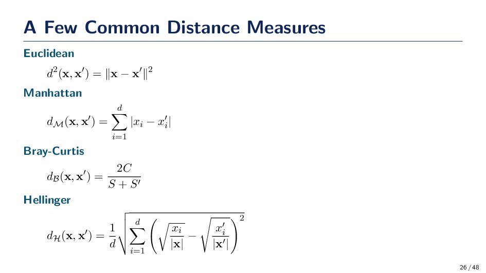
25. Choosing a Distance Measure Requirements: d(x, x′) ≥ 0, d(x, x′) + d(x′, z) ≥ d(x, z), d(x, x′) = d(x′, x) • The selection of the distance measure is a user defined parameter and leads to a wide selection of viable options • Results may vary significantly depending on the distance measure that is selected • As always, its up to the designer to select a measure that works • Can you think of some measures of distance? • Manhattan, Euclidean, Spearman, Hellinger, Chord, Bhattacharyya, Mahalanobis, Hamming, Jaccard, . . . • Is Kullback–Leibler divergence considered a distance as defined above? 25 / 48
26. A Few Common Distance Measures Euclidean d2(x, x′) = ∥x − x′∥2 Manhattan dM (x, x′) = d i=1 |xi − x′ i | Bray-Curtis dB (x, x′) = 2C S + S′ Hellinger dH (x, x′) = 1 d d i=1 xi |x| − x′ i |x′| 2 26 / 48
27. MDS Applied to MNIST 40 20 0 20 40 PC1 40 20 0 20 40 PC2 0 1 2 3 4 5 6 7 8 9 27 / 48
28. Feature Selection 28 / 48
29. Motivation What are the input variables that ∗best∗ describe an outcome? • Bacterial abundance profiles are collected from unhealthy and healthy patients. What are the bacteria that best differentiate between the two populations? • Observations of a variable are not free. Which variables should I “pay” for, possibly in the future, to build a classifier? 29 / 48
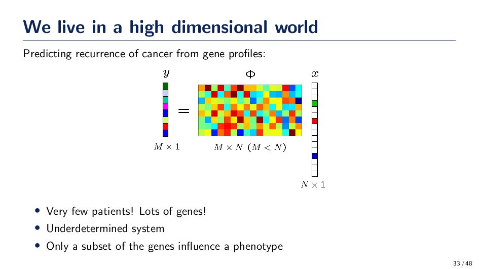
30. More about this high dimensional world Examples There are an ever increasing number of applications that generate high dimensional data! • Biometric authentication • Pharmaceutical industries • Systems biology • Geo-spatial data • Cancer diagnosis • Metagenomics 30 / 48
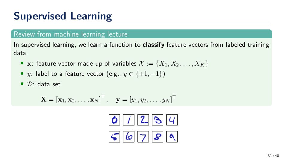
31. Supervised Learning Review from machine learning lecture In supervised learning, we learn a function to classify feature vectors from labeled training data. • x: feature vector made up of variables X := {X1 , X2 , . . . , XK } • y: label to a feature vector (e.g., y ∈ {+1, −1}) • D: data set X = [x1 , x2 , . . . , xN ]T , y = [y1 , y2 , . . . , yN ]T 31 / 48
32. Subset Selection! x 2 RK y 2 Y y = sign(wTx) −10 −8 −6 −4 −2 0 2 4 6 8 10 0 0.5 1 Strongly Relevant Irrelevant Weakly Relevant w0 w1 . . . wK . . . example! max J (X, y) x0 2 Rk 32 / 48
33. We live in a high dimensional world Predicting recurrence of cancer from gene profiles: • Very few patients! Lots of genes! • Underdetermined system • Only a subset of the genes influence a phenotype 33 / 48
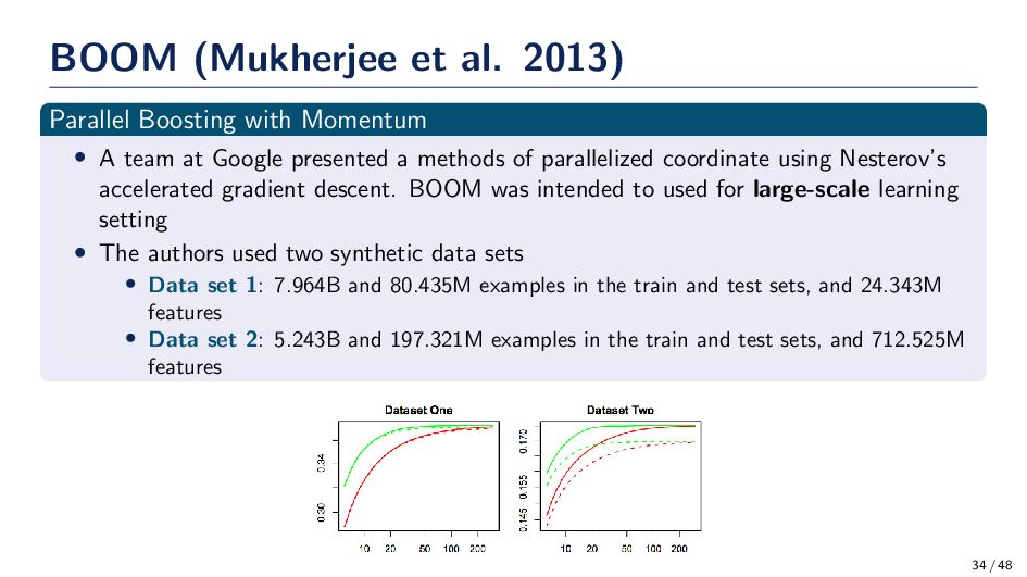
34. BOOM (Mukherjee et al. 2013) Parallel Boosting with Momentum • A team at Google presented a methods of parallelized coordinate using Nesterov’s accelerated gradient descent. BOOM was intended to used for large-scale learning setting • The authors used two synthetic data sets • Data set 1: 7.964B and 80.435M examples in the train and test sets, and 24.343M features • Data set 2: 5.243B and 197.321M examples in the train and test sets, and 712.525M features 34 / 48
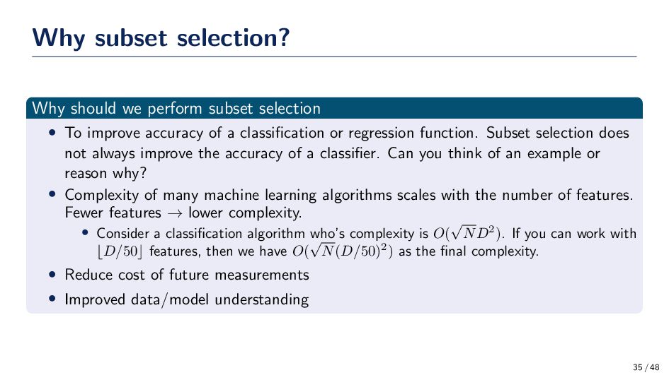
35. Why subset selection? Why should we perform subset selection • To improve accuracy of a classification or regression function. Subset selection does not always improve the accuracy of a classifier. Can you think of an example or reason why? • Complexity of many machine learning algorithms scales with the number of features. Fewer features → lower complexity. • Consider a classification algorithm who’s complexity is O( √ ND2). If you can work with ⌊D/50⌋ features, then we have O( √ N(D/50)2) as the final complexity. • Reduce cost of future measurements • Improved data/model understanding 35 / 48
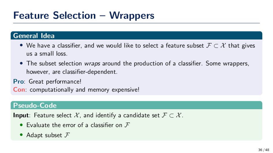
36. Feature Selection – Wrappers General Idea • We have a classifier, and we would like to select a feature subset F ⊂ X that gives us a small loss. • The subset selection wraps around the production of a classifier. Some wrappers, however, are classifier-dependent. Pro: Great performance! Con: computationally and memory expensive! Pseudo-Code Input: Feature select X, and identify a candidate set F ⊂ X. • Evaluate the error of a classifier on F • Adapt subset F 36 / 48
37. Question about the search space? If I have K features, how many different feature set combinations exist? Answer: 2K 37 / 48
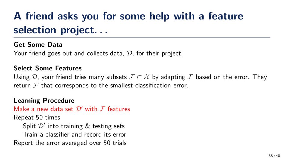
38. A friend asks you for some help with a feature selection project. . . Get Some Data Your friend goes out and collects data, D, for their project Select Some Features Using D, your friend tries many subsets F ⊂ X by adapting F based on the error. They return F that corresponds to the smallest classification error. Learning Procedure Make a new data set D′ with F features Repeat 50 times Split D′ into training & testing sets Train a classifier and record its error Report the error averaged over 50 trials 38 / 48
39. Feature selection is a part of the learning process Lui et al., “Feature Selection: An Ever Evolving Frontier in Data Mining,” in Workshop on Feature Selection in Data Mining, 2010. 39 / 48
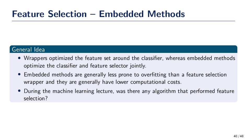
40. Feature Selection – Embedded Methods General Idea • Wrappers optimized the feature set around the classifier, whereas embedded methods optimize the classifier and feature selector jointly. • Embedded methods are generally less prone to overfitting than a feature selection wrapper and they are generally have lower computational costs. • During the machine learning lecture, was there any algorithm that performed feature selection? 40 / 48
41. Examples Least absolute shrinkage and selection operator (LASSO) β∗ = arg min β∈RK 1 2N ∥y − Xβ∥2 2 + λ∥β∥1 Elastic Nets β∗ = arg min β∈RK 1 2N ∥y − Xβ∥2 2 + 1 − α 2 ∥β∥2 2 + α∥β∥1 41 / 48
42. LASSO applied to some data 10−2 100 0 50 100 150 200 250 λ MSE 42 / 48
43. LASSO applied to some data 0 5 10 15 0 1 2 3 4 5 6 λ Non−zero coefficients 43 / 48
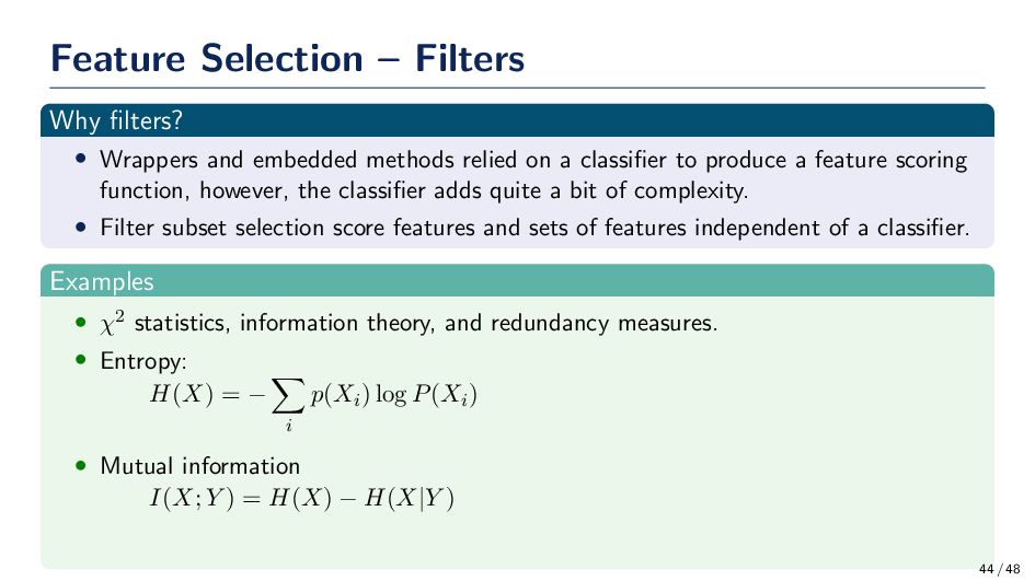
44. Feature Selection – Filters Why filters? • Wrappers and embedded methods relied on a classifier to produce a feature scoring function, however, the classifier adds quite a bit of complexity. • Filter subset selection score features and sets of features independent of a classifier. Examples • χ2 statistics, information theory, and redundancy measures. • Entropy: H(X) = − i p(Xi ) log P(Xi ) • Mutual information I(X; Y ) = H(X) − H(X|Y ) 44 / 48
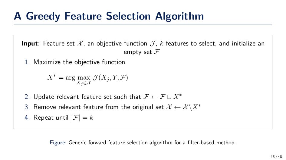
45. A Greedy Feature Selection Algorithm Input: Feature set X, an objective function J , k features to select, and initialize an empty set F 1. Maximize the objective function X∗ = arg max Xj∈X J (Xj , Y, F) 2. Update relevant feature set such that F ← F ∪ X∗ 3. Remove relevant feature from the original set X ← X\X∗ 4. Repeat until |F| = k Figure: Generic forward feature selection algorithm for a filter-based method. 45 / 48
46. Information theoretic objective functions Mutual Information Maximization (MIM) J (Xk , Y ) = I(Xk ; Y ) minimum Redundancy Maximum Relevancy (mRMR) J (Xk , Y, F) = I(Xk ; Y ) − 1 |F| Xj∈F I(Xk ; Xj ) Joint Mutual Information (JMI) J (Xk , Y, F) = I(Xk ; Y ) − 1 |F| Xj∈F (I(Xk ; Xj ) − I(Xk ; Xj |Y )) 46 / 48
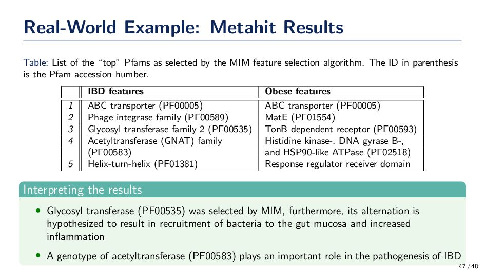
47. Real-World Example: Metahit Results Table: List of the “top” Pfams as selected by the MIM feature selection algorithm. The ID in parenthesis is the Pfam accession humber. IBD features Obese features 1 ABC transporter (PF00005) ABC transporter (PF00005) 2 Phage integrase family (PF00589) MatE (PF01554) 3 Glycosyl transferase family 2 (PF00535) TonB dependent receptor (PF00593) 4 Acetyltransferase (GNAT) family Histidine kinase-, DNA gyrase B-, (PF00583) and HSP90-like ATPase (PF02518) 5 Helix-turn-helix (PF01381) Response regulator receiver domain Interpreting the results • Glycosyl transferase (PF00535) was selected by MIM, furthermore, its alternation is hypothesized to result in recruitment of bacteria to the gut mucosa and increased inflammation • A genotype of acetyltransferase (PF00583) plays an important role in the pathogenesis of IBD 47 / 48
48. The End 48 / 48