capturing uncertainty in data, our estimators and our models. It is critical to understand probability and how it plays into us making decisions. • How does probability play into risk and decision making? Obviously we want to make decisions that lead to the smallest amount of risk. • What assumptions do we need to make? • Generating data from probability distributions is valuable to benchmark algorithms we learn about or develop. • Bayes decision theory set up the foundation we need to pursue a concrete understanding of machine learning. 4 / 45
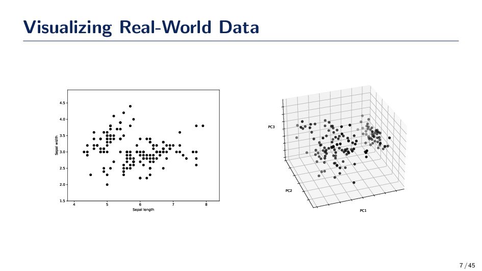
aspect will encounter in machine learning is benchmarking our algorithms and the data we use in the experiment are very important • Real-world data are the true test to a model’s performance but obtaining such data can be hard and expensive • Synthetic data can provide us a way to “know” the ground truth for data • How should we generate data if we want to do a simple classification problem? What distribution should we use? • What if I want to calculate p(X), p(X|Y ), or p(Y )? 6 / 45
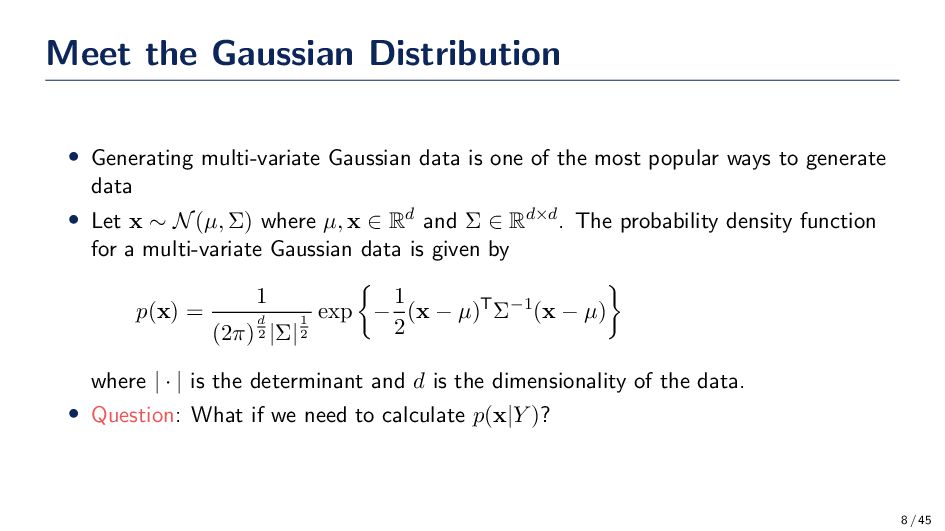
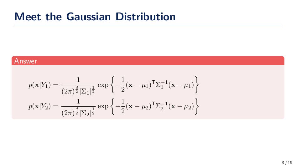
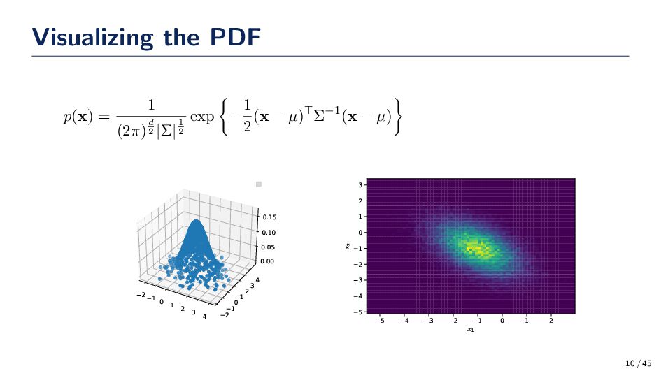
one of the most popular ways to generate data • Let x ∼ N(µ, Σ) where µ, x ∈ Rd and Σ ∈ Rd×d. The probability density function for a multi-variate Gaussian data is given by p(x) = 1 (2π)d 2 |Σ|1 2 exp − 1 2 (x − µ)TΣ−1(x − µ) where | · | is the determinant and d is the dimensionality of the data. • Question: What if we need to calculate p(x|Y )? 8 / 45
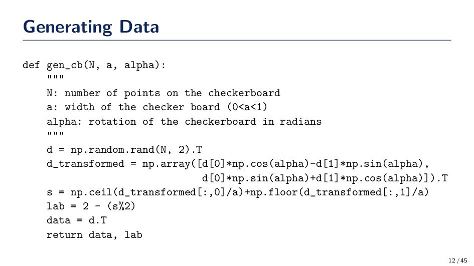
points on the checkerboard a: width of the checker board (0<a<1) alpha: rotation of the checkerboard in radians """ d = np.random.rand(N, 2).T d_transformed = np.array([d[0]*np.cos(alpha)-d[1]*np.sin(alpha), d[0]*np.sin(alpha)+d[1]*np.cos(alpha)]).T s = np.ceil(d_transformed[:,0]/a)+np.floor(d_transformed[:,1]/a) lab = 2 - (s%2) data = d.T return data, lab 12 / 45
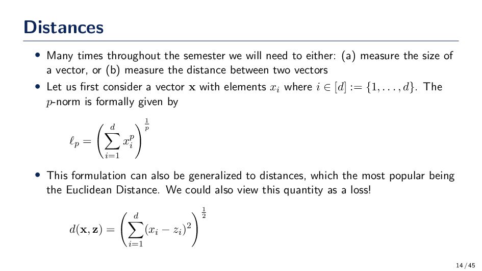
to either: (a) measure the size of a vector, or (b) measure the distance between two vectors • Let us first consider a vector x with elements xi where i ∈ [d] := {1, . . . , d}. The p-norm is formally given by ℓp = d i=1 xp i 1 p • This formulation can also be generalized to distances, which the most popular being the Euclidean Distance. We could also view this quantity as a loss! d(x, z) = d i=1 (xi − zi )2 1 2 14 / 45
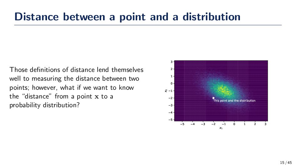
distance lend themselves well to measuring the distance between two points; however, what if we want to know the “distance” from a point x to a probability distribution? 5 4 3 2 1 0 1 2 3 x1 5 4 3 2 1 0 1 2 3 x2 This point and the distribution 15 / 45
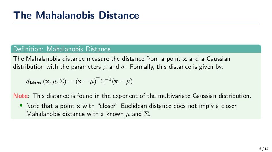
the distance from a point x and a Gaussian distribution with the parameters µ and σ. Formally, this distance is given by: dMahal (x, µ, Σ) = (x − µ)TΣ−1(x − µ) Note: This distance is found in the exponent of the multivariate Gaussian distribution. • Note that a point x with “closer” Euclidean distance does not imply a closer Mahalanobis distance with a known µ and Σ. 16 / 45
of possible outcomes for the random experiment • Events (F): the set of possible events for the random experiment • Probability (P): a function P : F → [0, 1] assigning a number P(A) ∈ [0, 1] to each A ∈ F, satisfying the axioms of probability given later in this section. • Laws of Probability • Non-negativity: P(A) ≥ 0 for all A ∈ F. • Additivity: if A, B are disjoint events (A ∩ B = ∅) then P(A ∪ B) = P(A) + P(B). More generally if |Ω| = inf and {A1 , A2 , . . .} is an infinite sequence of disjoint events, then P(A1 ∪ A2 ∪ · · · ) = P(A1 ) + P(A2 ) + · · · • Normalization: P(Ω) = 1 (something must happen) 18 / 45
variable can always be obtained by summing (integrating) the probability density function (pdf) over all values of all other variables. For example, P(X) = Y ∈Y P(X, Y ) P(X) = Z∈Z Y ∈Y P(X, Y, Z) 19 / 45
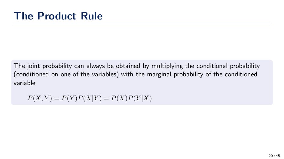
by multiplying the conditional probability (conditioned on one of the variables) with the marginal probability of the conditioned variable P(X, Y ) = P(Y )P(X|Y ) = P(X)P(Y |X) 20 / 45
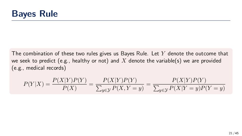
Bayes Rule. Let Y denote the outcome that we seek to predict (e.g., healthy or not) and X denote the variable(s) we are provided (e.g., medical records) P(Y |X) = P(X|Y )P(Y ) P(X) = P(X|Y )P(Y ) y∈Y P(X, Y = y) = P(X|Y )P(Y ) y∈Y P(X|Y = y)P(Y = y) 21 / 45
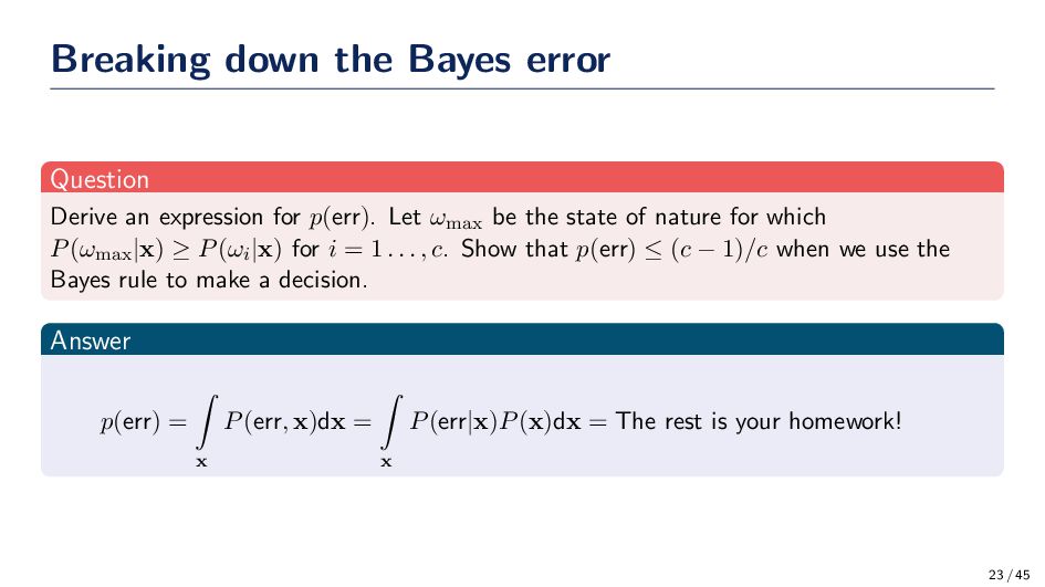
p(err). Let ωmax be the state of nature for which P(ωmax |x) ≥ P(ωi |x) for i = 1 . . . , c. Show that p(err) ≤ (c − 1)/c when we use the Bayes rule to make a decision. Answer p(err) = x P(err, x)dx = x P(err|x)P(x)dx = The rest is your homework! 23 / 45
kids now grown into adults. Obviously there is me, Greg. I was born on a Wednesday. What is the probability that I have a brother? You can assume that P(boy) = P(girl) = 1 2 . 25 / 45
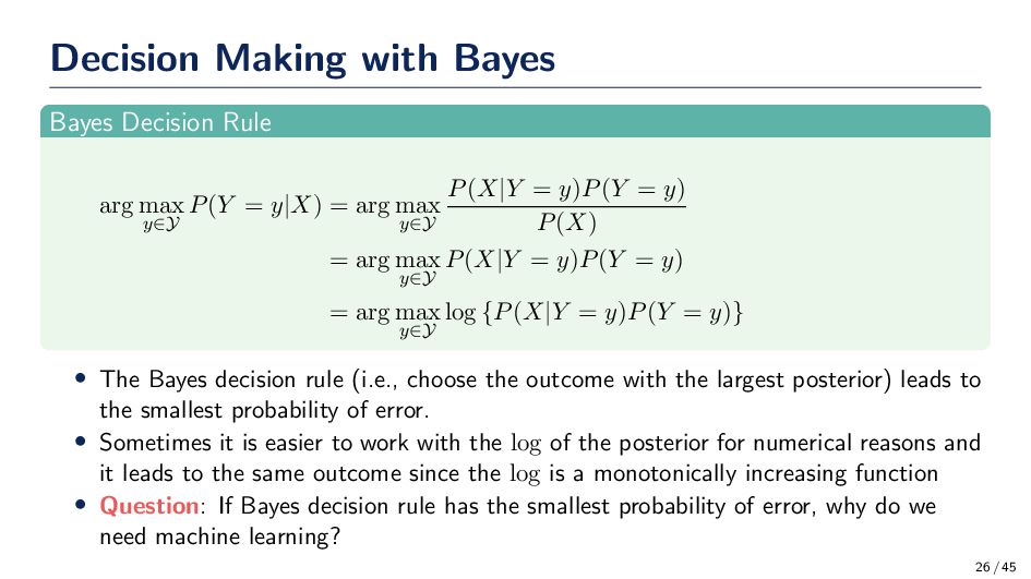
P(Y = y|X) = arg max y∈Y P(X|Y = y)P(Y = y) P(X) = arg max y∈Y P(X|Y = y)P(Y = y) = arg max y∈Y log {P(X|Y = y)P(Y = y)} • The Bayes decision rule (i.e., choose the outcome with the largest posterior) leads to the smallest probability of error. • Sometimes it is easier to work with the log of the posterior for numerical reasons and it leads to the same outcome since the log is a monotonically increasing function • Question: If Bayes decision rule has the smallest probability of error, why do we need machine learning? 26 / 45
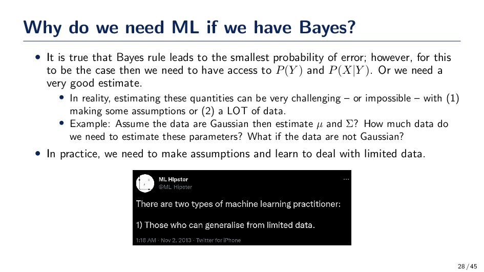
It is true that Bayes rule leads to the smallest probability of error; however, for this to be the case then we need to have access to P(Y ) and P(X|Y ). Or we need a very good estimate. • In reality, estimating these quantities can be very challenging – or impossible – with (1) making some assumptions or (2) a LOT of data. • Example: Assume the data are Gaussian then estimate µ and Σ? How much data do we need to estimate these parameters? What if the data are not Gaussian? • In practice, we need to make assumptions and learn to deal with limited data. 28 / 45
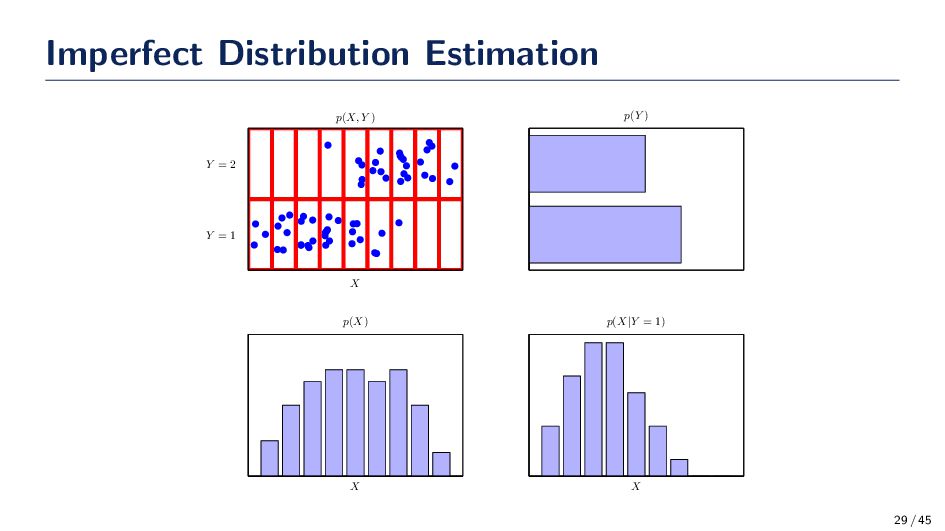
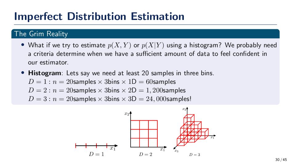
try to estimate p(X, Y ) or p(X|Y ) using a histogram? We probably need a criteria determine when we have a sufficient amount of data to feel confident in our estimator. • Histogram: Lets say we need at least 20 samples in three bins. D = 1 : n = 20samples × 3bins × 1D = 60samples D = 2 : n = 20samples × 3bins × 2D = 1, 200samples D = 3 : n = 20samples × 3bins × 3D = 24, 000samples! x1 D = 1 x1 x2 D = 2 x1 x2 x3 D = 3 30 / 45
estimate a density in 1D to 24,000 samples in 3D! Imagine what happens if we went to 50D! The Curse of Dimensionality • The severe difficulty that can arise in spaces of many dimensions is sometimes called the curse of dimensionality (Bellman, 1961) • Bellman R. (1961) “Adaptive Control Processes.” Princeton University Press, Princeton, NJ. • Although this is now a power law growth, rather than an exponential growth, it still points to the method becoming rapidly unwieldy and of limited practical utility • You have been be warned, however, that not all intuitions developed in spaces of low dimensionality will generalize to spaces of many dimensions 31 / 45
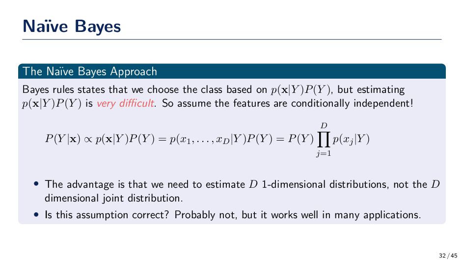
states that we choose the class based on p(x|Y )P(Y ), but estimating p(x|Y )P(Y ) is very difficult. So assume the features are conditionally independent! P(Y |x) ∝ p(x|Y )P(Y ) = p(x1 , . . . , xD |Y )P(Y ) = P(Y ) D j=1 p(xj |Y ) • The advantage is that we need to estimate D 1-dimensional distributions, not the D dimensional joint distribution. • Is this assumption correct? Probably not, but it works well in many applications. 32 / 45
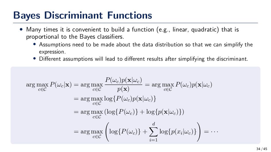
build a function (e.g., linear, quadratic) that is proportional to the Bayes classifiers. • Assumptions need to be made about the data distribution so that we can simplify the expression. • Different assumptions will lead to different results after simplifying the discriminant. arg max c∈C P(ωc |x) = arg max c∈C P(ωc )p(x|ωc ) p(x) = arg max c∈C P(ωc )p(x|ωc ) = arg max c∈C log{P(ωc )p(x|ωc )} = arg max c∈C (log{P(ωc )} + log{p(x|ωc )}) = arg max c∈C log{P(ωc )} + d i=1 log{p(xi |ωc )} = · · · 34 / 45
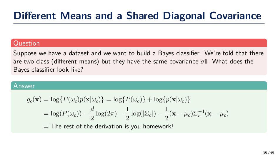
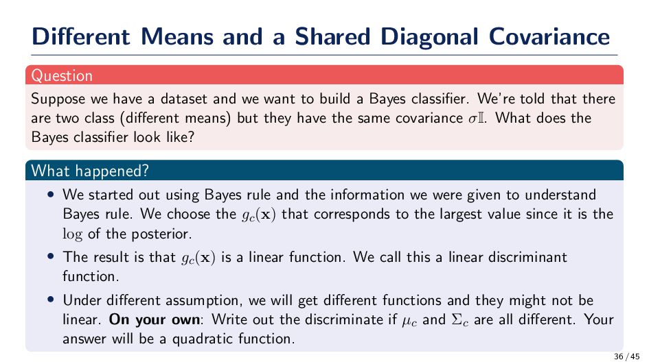
have a dataset and we want to build a Bayes classifier. We’re told that there are two class (different means) but they have the same covariance σI. What does the Bayes classifier look like? Answer gc (x) = log{P(ωc )p(x|ωc )} = log{P(ωc )} + log{p(x|ωc )} = log(P(ωc )) − d 2 log(2π) − 1 2 log(|Σc |) − 1 2 (x − µc )Σ−1 c (x − µc ) = The rest of the derivation is you homework! 35 / 45
have a dataset and we want to build a Bayes classifier. We’re told that there are two class (different means) but they have the same covariance σI. What does the Bayes classifier look like? What happened? • We started out using Bayes rule and the information we were given to understand Bayes rule. We choose the gc (x) that corresponds to the largest value since it is the log of the posterior. • The result is that gc (x) is a linear function. We call this a linear discriminant function. • Under different assumption, we will get different functions and they might not be linear. On your own: Write out the discriminate if µc and Σc are all different. Your answer will be a quadratic function. 36 / 45
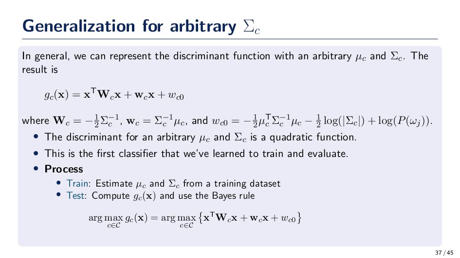
discriminant function with an arbitrary µc and Σc. The result is gc (x) = xTWcx + wcx + wc0 where Wc = −1 2 Σ−1 c , wc = Σ−1 c µc, and wc0 = −1 2 µT c Σ−1 c µc − 1 2 log(|Σc |) + log(P(ωj )). • The discriminant for an arbitrary µc and Σc is a quadratic function. • This is the first classifier that we’ve learned to train and evaluate. • Process • Train: Estimate µc and Σc from a training dataset • Test: Compute gc (x) and use the Bayes rule arg max c∈C gc (x) = arg max c∈C xTWc x + wc x + wc0 37 / 45
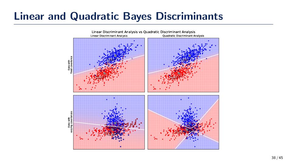
Discriminant Analysis Quadratic Discriminant Analysis Data with varying covariances Linear Discriminant Analysis vs Quadratic Discriminant Analysis 38 / 45
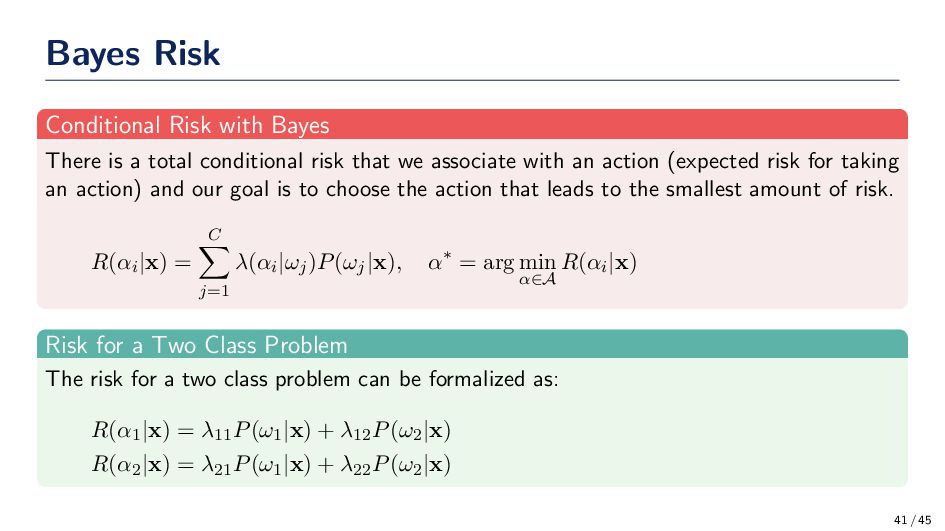
section of the lecture is to understand the risk we take when a decision is made. Obviously, we want to make decisions that lead to the smallest amount of risk. Definitions • Classes: {ω1 , . . . , ωC }. • Actions: {α1 , . . . , αℓ }. Note that ℓ need not equal C. • Cost: {λ1 , . . . , λℓ }. • Cost Function: λ(αi |ωj ): Cost of taking action αi when the state of nature is ωj. 40 / 45
conditional risk that we associate with an action (expected risk for taking an action) and our goal is to choose the action that leads to the smallest amount of risk. R(αi |x) = C j=1 λ(αi |ωj )P(ωj |x), α∗ = arg min α∈A R(αi |x) Risk for a Two Class Problem The risk for a two class problem can be formalized as: R(α1 |x) = λ11 P(ω1 |x) + λ12 P(ω2 |x) R(α2 |x) = λ21 P(ω1 |x) + λ22 P(ω2 |x) 41 / 45
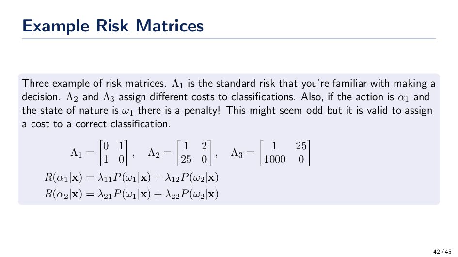
the standard risk that you’re familiar with making a decision. Λ2 and Λ3 assign different costs to classifications. Also, if the action is α1 and the state of nature is ω1 there is a penalty! This might seem odd but it is valid to assign a cost to a correct classification. Λ1 = 0 1 1 0 , Λ2 = 1 2 25 0 , Λ3 = 1 25 1000 0 R(α1 |x) = λ11 P(ω1 |x) + λ12 P(ω2 |x) R(α2 |x) = λ21 P(ω1 |x) + λ22 P(ω2 |x) 42 / 45
uncertainty in data and outcomes. Effectively capturing uncertainty is crucial in nearly all applications of machine learning. • The curse of dimensionality is a serious limitation and motivates us to pursue other data-driven methods to decision making that are inspired by Bayes and optimization. 43 / 45
![Machine Learning Lectures Decision Making with Bayes Gregory Ditzler [email protected]](https://files.speakerdeck.com/presentations/59be63f16c364a0bb8c60271a8d56334/slide_0.jpg)