Machine Learning Lectures - MLPs

Transcript

1. Machine Learning Lectures Multilayer Perceptrons and Backpropagation Gregory Ditzler gregory.ditzler@gmail.com February 24, 2024 1 / 47
2. Overview 1. Motivation 2. A Brief History of Neural Networks 3. The Multilayer Perceptron and Backpropagation 2 / 47
3. Motivation 3 / 47
4. Lecture Overview • Our goal is the develop an understanding of how neural networks work and how they can be trained. • Neural networks are universal approximators. The universal approximation theorem implies that neural networks can represent a wide variety of functions when given appropriate weights. They typically do not provide a construction for the weights, but merely state that such a construction is possible. 4 / 47
5. A Brief History of Neural Networks 5 / 47
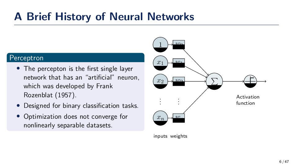
6. A Brief History of Neural Networks Perceptron • The percepton is the first single layer network that has an “artificial” neuron, which was developed by Frank Rozenblat (1957). • Designed for binary classification tasks. • Optimization does not converge for nonlinearly separable datasets. Activation function w2 x2 . . . . . . wn xn w1 x1 w0 1 inputs weights 6 / 47
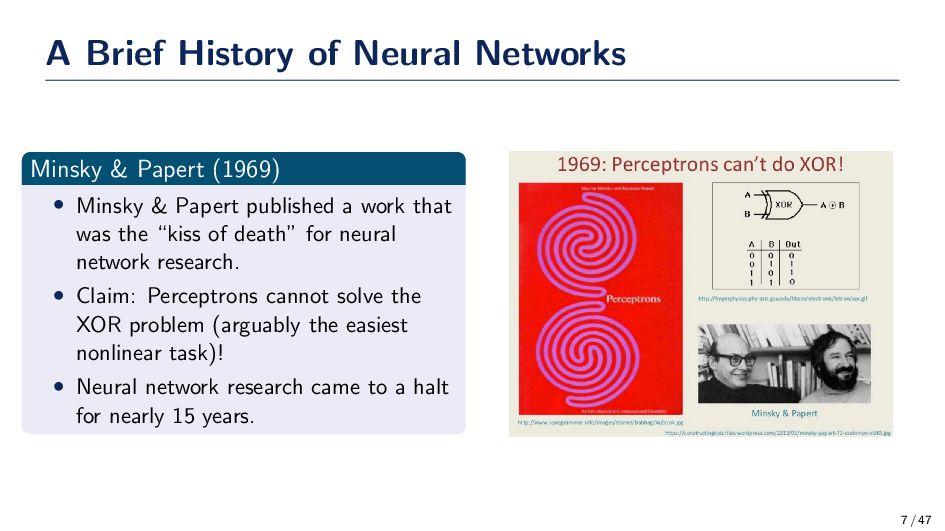
7. A Brief History of Neural Networks Minsky & Papert (1969) • Minsky & Papert published a work that was the “kiss of death” for neural network research. • Claim: Perceptrons cannot solve the XOR problem (arguably the easiest nonlinear task)! • Neural network research came to a halt for nearly 15 years. 7 / 47
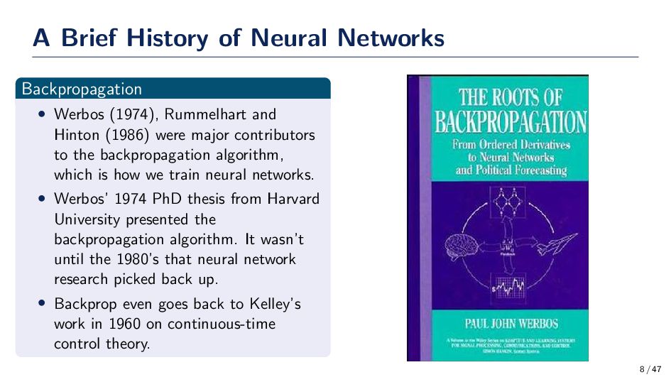
8. A Brief History of Neural Networks Backpropagation • Werbos (1974), Rummelhart and Hinton (1986) were major contributors to the backpropagation algorithm, which is how we train neural networks. • Werbos’ 1974 PhD thesis from Harvard University presented the backpropagation algorithm. It wasn’t until the 1980’s that neural network research picked back up. • Backprop even goes back to Kelley’s work in 1960 on continuous-time control theory. 8 / 47
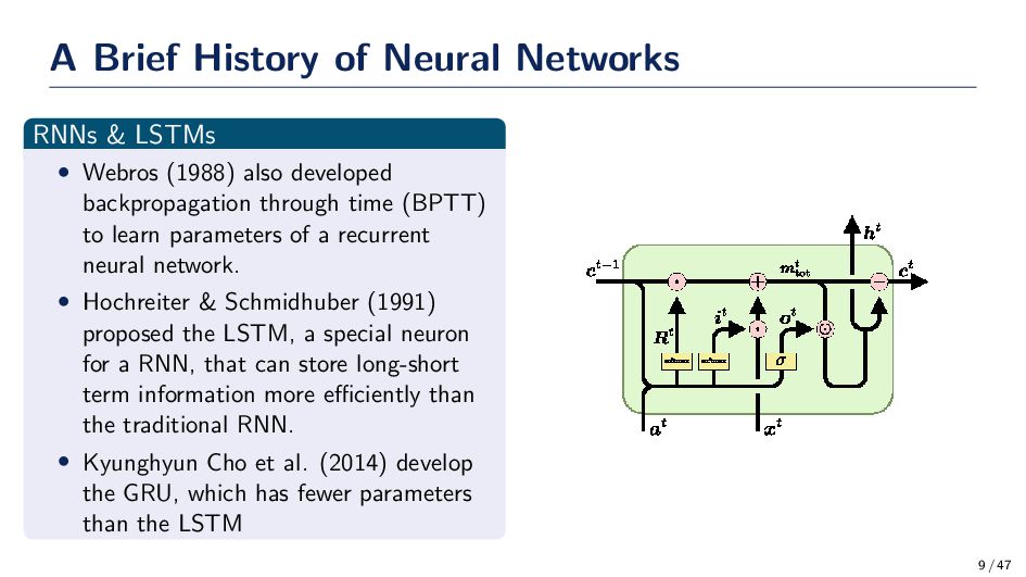
9. A Brief History of Neural Networks RNNs & LSTMs • Webros (1988) also developed backpropagation through time (BPTT) to learn parameters of a recurrent neural network. • Hochreiter & Schmidhuber (1991) proposed the LSTM, a special neuron for a RNN, that can store long-short term information more efficiently than the traditional RNN. • Kyunghyun Cho et al. (2014) develop the GRU, which has fewer parameters than the LSTM 9 / 47
10. A Brief History of Neural Networks CNNs • Le Cunn et al. developed the convolutional neural network. These networks are efficient at classify images where spatial information can be captured. 10 / 47
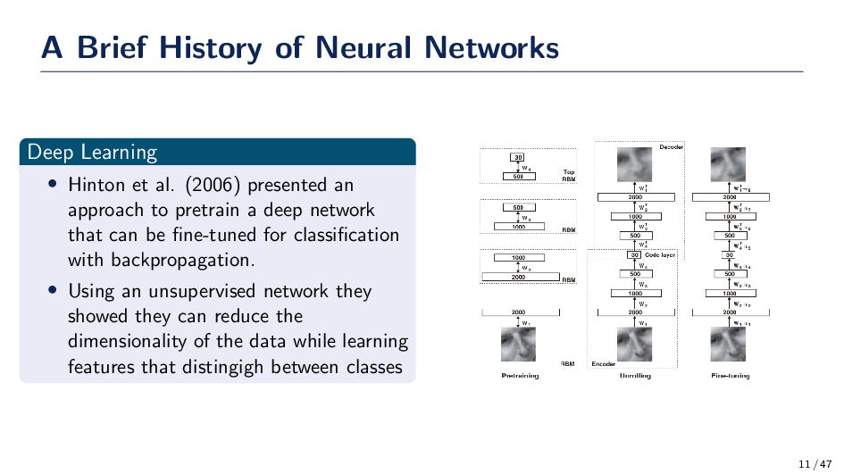
11. A Brief History of Neural Networks Deep Learning • Hinton et al. (2006) presented an approach to pretrain a deep network that can be fine-tuned for classification with backpropagation. • Using an unsupervised network they showed they can reduce the dimensionality of the data while learning features that distingigh between classes 11 / 47
12. A Brief History of Neural Networks Deep Learning and Beyond • GANs: DC-GAN, C-GAN, AC-GAN, Cyle GAN, InfoGAN, etc. • Variantions: DenseNet, MobileNet, VGG16/19, Resnet, etc. 12 / 47
13. The Multilayer Perceptron and Backpropagation 13 / 47
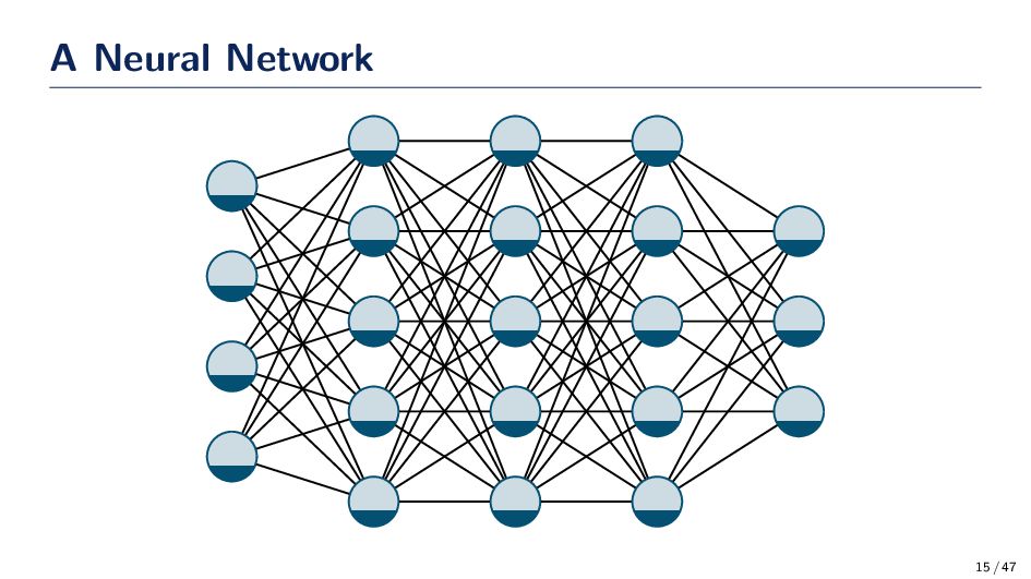
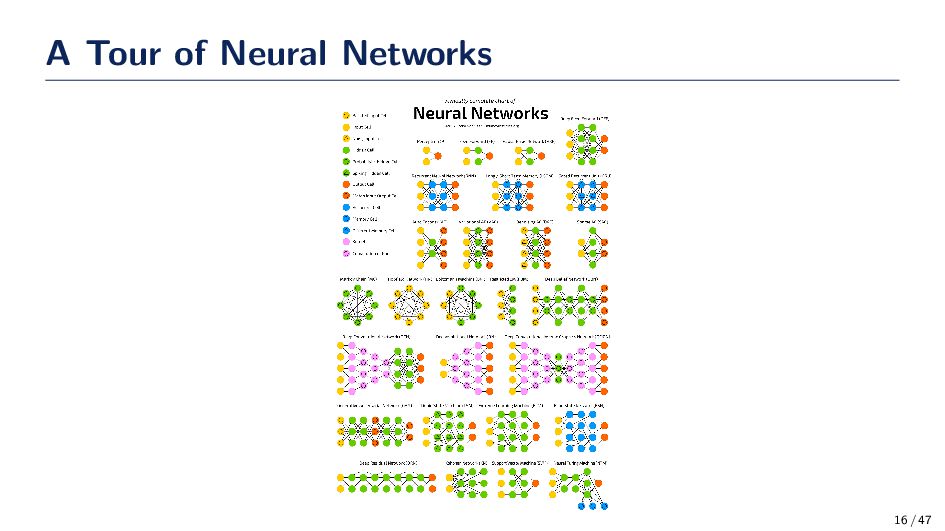
14. Definitions MSFT Encarta A neural network is a highly interconnected network of information-processing elements that mimics the connectivity and functioning of the human brain. One of the most significant strengths of neural networks is their ability to learn from a limited set of examples. 14 / 47
15. A Neural Network 15 / 47
16. A Tour of Neural Networks 16 / 47
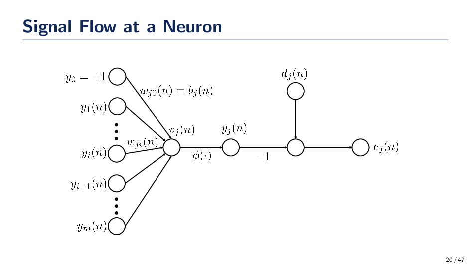
17. Definitions • We assume a supervised learning setting where we’re provided a training data set D := {x(n), d(n)}N n=1 , where x(n) is a feature vector and d(n) is the desired output for the nth sample. • Notation such as dj (n) is used to refer to the jth output node of the desired signal • Neuron and node are used interchangeably • The first and last layers of the network are referred to as the input and output layer, respectively. All layers between the input and output are referred to as hidden layers. • For the moment, we’re only going to exam a neural network with one hidden layer; however, we can generalize the results to multiple hidden layers. • Training a very deep network can be challenging due to issues we cover in this lecture and future lectures will address training a deep network. 17 / 47
18. Definitions The Credit Assignment Problem • The credit assignment problem is one where we seek to credit or blame for overall outcomes to each of the internal decisions made by the hidden computational units. • These hidden units are the first to “blame” for an error made at the output because the data are processed internally before ever reaching the output. • How much “weight” or “credit” do we assign a neuron when an error is made at the output? • The backpropagation algorithm solves the credit assignment problem in an elegant manner. 18 / 47
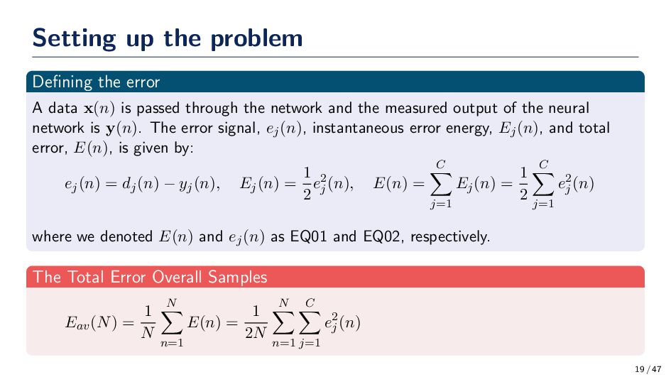
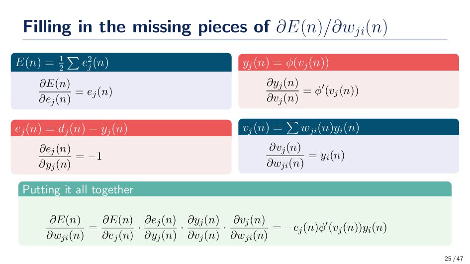
19. Setting up the problem Defining the error A data x(n) is passed through the network and the measured output of the neural network is y(n). The error signal, ej(n), instantaneous error energy, Ej(n), and total error, E(n), is given by: ej(n) = dj(n) − yj(n), Ej(n) = 1 2 e2 j (n), E(n) = C j=1 Ej(n) = 1 2 C j=1 e2 j (n) where we denoted E(n) and ej(n) as EQ01 and EQ02, respectively. The Total Error Overall Samples Eav(N) = 1 N N n=1 E(n) = 1 2N N n=1 C j=1 e2 j (n) 19 / 47
20. Signal Flow at a Neuron … … 20 / 47
21. Signal Flow at a Neuron The induced local field, vj(n) is produced at the input of the activation associated with neuron j, which is given by: vj(n) = m i=1 wji(n)yi(n) The signal at the neuron is yj(n) = ϕ(vj(n)) where ϕ(·) is a nonlinear activation function. We refer to yj(n) and vj(n) as EQ3 and EQ4, respectively. 21 / 47
22. Example Activation Functions 3 2 1 0 1 2 3 1.5 1.0 0.5 0.0 0.5 1.0 1.5 Relu LeakyRelu Sigmoid Tanh 22 / 47
23. Setting up gradient descent Keeping our eye on the prize Out goal is to determine the update rule for the weights of the neural network using gradient descent. Therefore, we need to find the gradient of the error w.r.t. the parameters w. Recall that the update for gradient descent is given by: w(t + 1) = w(t) + ∆w(t) = w(t) − η ∂E ∂w We have a problem! The term w does not show up in the expression for E, which makes finding ∂E ∂w more challenging. Finding the gradient is going to be very difficult unless we look at the problem differently. 23 / 47
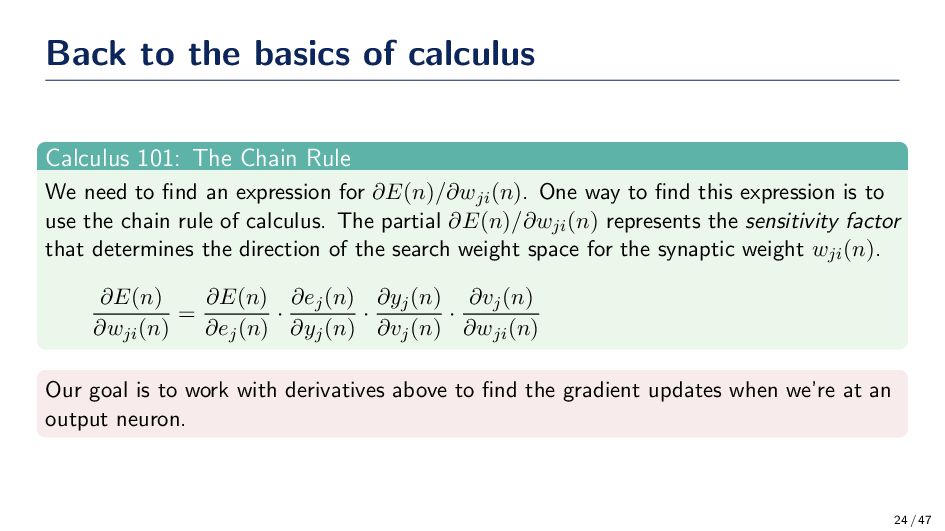
24. Back to the basics of calculus Calculus 101: The Chain Rule We need to find an expression for ∂E(n)/∂wji(n). One way to find this expression is to use the chain rule of calculus. The partial ∂E(n)/∂wji(n) represents the sensitivity factor that determines the direction of the search weight space for the synaptic weight wji(n). ∂E(n) ∂wji(n) = ∂E(n) ∂ej(n) · ∂ej(n) ∂yj(n) · ∂yj(n) ∂vj(n) · ∂vj(n) ∂wji(n) Our goal is to work with derivatives above to find the gradient updates when we’re at an output neuron. 24 / 47
25. Filling in the missing pieces of ∂E(n)/∂wji (n) E(n) = 1 2 e2 j (n) ∂E(n) ∂ej(n) = ej(n) ej (n) = dj (n) − yj (n) ∂ej(n) ∂yj(n) = −1 yj (n) = ϕ(vj (n)) ∂yj(n) ∂vj(n) = ϕ′(vj(n)) vj (n) = wji (n)yi (n) ∂vj(n) ∂wji(n) = yi(n) Putting it all together ∂E(n) ∂wji(n) = ∂E(n) ∂ej(n) · ∂ej(n) ∂yj(n) · ∂yj(n) ∂vj(n) · ∂vj(n) ∂wji(n) = −ej(n)ϕ′(vj(n))yi(n) 25 / 47
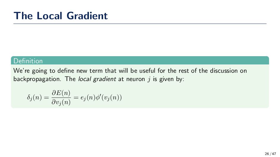
26. The Local Gradient Definition We’re going to define new term that will be useful for the rest of the discussion on backpropagation. The local gradient at neuron j is given by: δj(n) = ∂E(n) ∂vj(n) = ej(n)ϕ′(vj(n)) 26 / 47
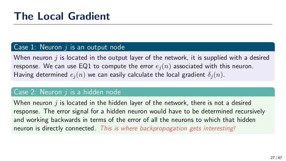
27. The Local Gradient Case 1: Neuron j is an output node When neuron j is located in the output layer of the network, it is supplied with a desired response. We can use EQ1 to compute the error ej(n) associated with this neuron. Having determined ej(n) we can easily calculate the local gradient δj(n). Case 2: Neuron j is a hidden node When neuron j is located in the hidden layer of the network, there is not a desired response. The error signal for a hidden neuron would have to be determined recursively and working backwards in terms of the error of all the neurons to which that hidden neuron is directly connected. This is where backpropogation gets interesting! 27 / 47
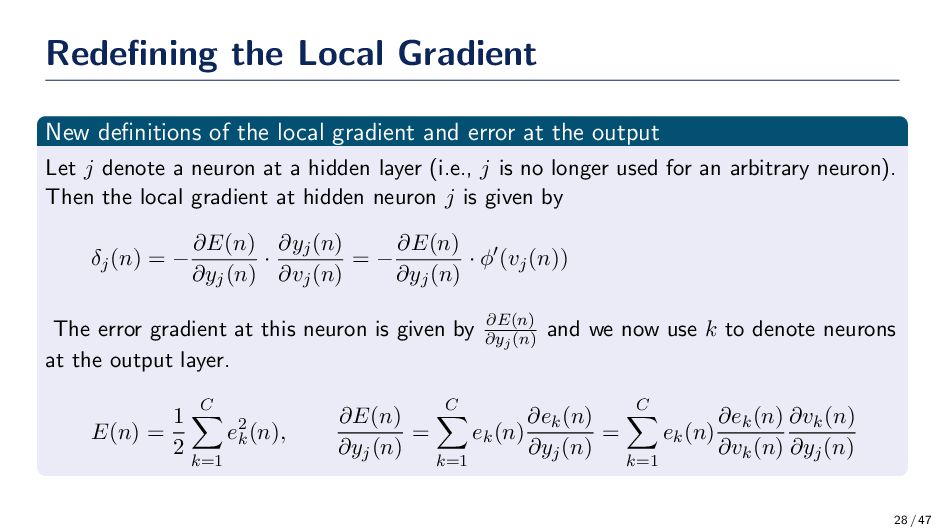
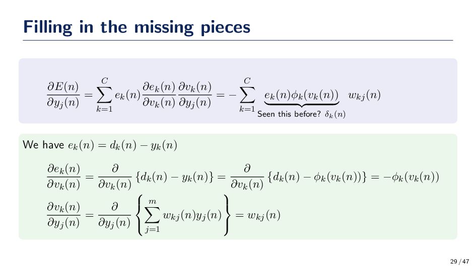
28. Redefining the Local Gradient New definitions of the local gradient and error at the output Let j denote a neuron at a hidden layer (i.e., j is no longer used for an arbitrary neuron). Then the local gradient at hidden neuron j is given by δj(n) = − ∂E(n) ∂yj(n) · ∂yj(n) ∂vj(n) = − ∂E(n) ∂yj(n) · ϕ′(vj(n)) The error gradient at this neuron is given by ∂E(n) ∂yj(n) and we now use k to denote neurons at the output layer. E(n) = 1 2 C k=1 e2 k (n), ∂E(n) ∂yj(n) = C k=1 ek(n) ∂ek(n) ∂yj(n) = C k=1 ek(n) ∂ek(n) ∂vk(n) ∂vk(n) ∂yj(n) 28 / 47
29. Filling in the missing pieces ∂E(n) ∂yj(n) = C k=1 ek(n) ∂ek(n) ∂vk(n) ∂vk(n) ∂yj(n) = − C k=1 ek(n)ϕk(vk(n)) Seen this before? δk(n) wkj(n) We have ek(n) = dk(n) − yk(n) ∂ek(n) ∂vk(n) = ∂ ∂vk(n) {dk(n) − yk(n)} = ∂ ∂vk(n) {dk(n) − ϕk(vk(n))} = −ϕk(vk(n)) ∂vk(n) ∂yj(n) = ∂ ∂yj(n)    m j=1 wkj(n)yj(n)    = wkj(n) 29 / 47
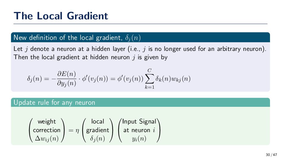
30. The Local Gradient New definition of the local gradient, δj (n) Let j denote a neuron at a hidden layer (i.e., j is no longer used for an arbitrary neuron). Then the local gradient at hidden neuron j is given by δj(n) = − ∂E(n) ∂yj(n) · ϕ′(vj(n)) = ϕ′(vj(n)) C k=1 δk(n)wkj(n) Update rule for any neuron   weight correction ∆wij(n)   = η   local gradient δj(n)     Input Signal at neuron i yi(n)   30 / 47
31. Example: MNIST Ground Truth: 3 Ground Truth: 9 Ground Truth: 4 Ground Truth: 9 Ground Truth: 9 Ground Truth: 0 31 / 47
32. Example: MNIST 0 25000 50000 75000 100000 125000 150000 175000 number of training examples seen 0.0 0.5 1.0 1.5 2.0 negative log likelihood loss Train Loss Test Loss 32 / 47
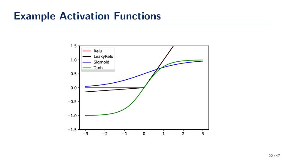
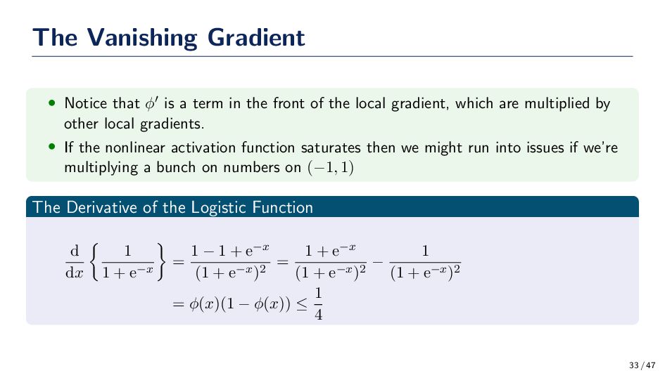
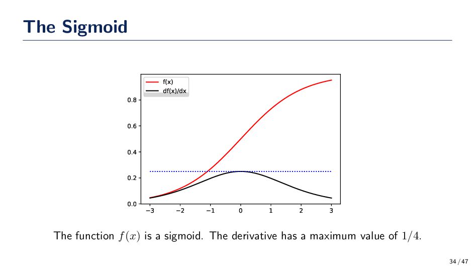
33. The Vanishing Gradient • Notice that ϕ′ is a term in the front of the local gradient, which are multiplied by other local gradients. • If the nonlinear activation function saturates then we might run into issues if we’re multiplying a bunch on numbers on (−1, 1) The Derivative of the Logistic Function d dx 1 1 + e−x = 1 − 1 + e−x (1 + e−x)2 = 1 + e−x (1 + e−x)2 − 1 (1 + e−x)2 = ϕ(x)(1 − ϕ(x)) ≤ 1 4 33 / 47
34. The Sigmoid 3 2 1 0 1 2 3 0.0 0.2 0.4 0.6 0.8 f(x) df(x)/dx The function f(x) is a sigmoid. The derivative has a maximum value of 1/4. 34 / 47
35. Consequences of the Vanishing Gradient • The multiplication of the local gradients (and ones coming from the previous layer) can cause the gradient to effectively vanish by the time the updates are done at layers close to the input. • Using backpropagation alone is not enough to train a deep multilayer perceptron. We’re going to need a different view of training deep neural network with an MLP. • Relu-like activation functions can help; however, changing the activation function is not going to be sufficient to effectively train a deep net. • Future lectures cover how to effectively train deep nets, but the main take away here is that backpropagation works well at training shallow nets; however, not deep nets. 35 / 47
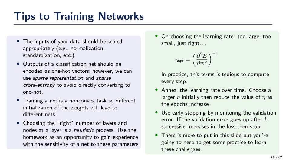
36. Tips to Training Networks • The inputs of your data should be scaled appropriately (e.g., normalization, standardization, etc.) • Outputs of a classification net should be encoded as one-hot vectors; however, we can use sparse representation and sparse cross-entropy to avoid directly converting to one-hot. • Training a net is a nonconvex task so different initialization of the weights will lead to different nets. • Choosing the “right” number of layers and nodes at a layer is a heuristic process. Use the homework as an opportunity to gain experience with the sensitivity of a net to these parameters • On choosing the learning rate: too large, too small, just right. . . ηopt = ∂2E ∂w2 −1 In practice, this terms is tedious to compute every step. • Anneal the learning rate over time. Choose a larger η initially then reduce the value of η as the epochs increase • Use early stopping by monitoring the validation error. If the validation error goes up after k successive increases in the loss then stop! • There is more to put in this slide but you’re going to need to get some practice to learn these challenges. 36 / 47
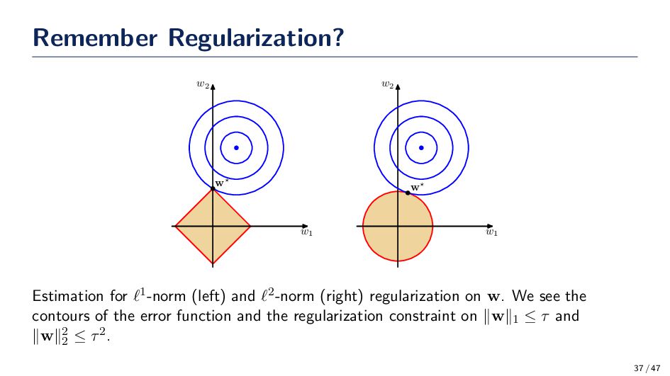
37. Remember Regularization? w1 w2 w w1 w2 w Estimation for ℓ1-norm (left) and ℓ2-norm (right) regularization on w. We see the contours of the error function and the regularization constraint on ∥w∥1 ≤ τ and ∥w∥2 2 ≤ τ2. 37 / 47
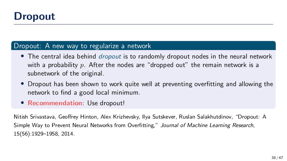
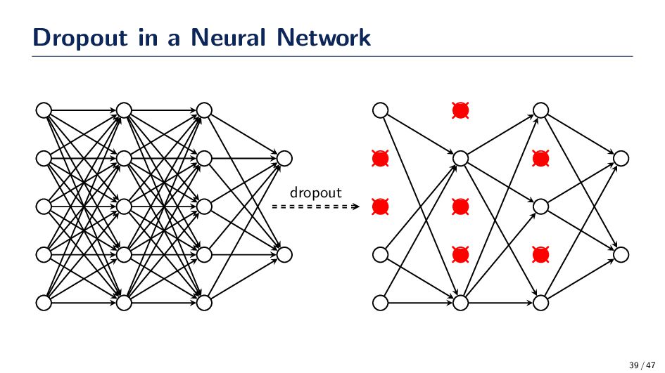
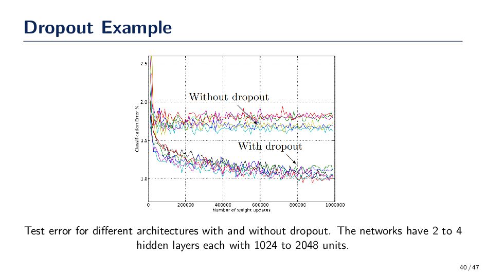
38. Dropout Dropout: A new way to regularize a network • The central idea behind dropout is to randomly dropout nodes in the neural network with a probability p. After the nodes are “dropped out” the remain network is a subnetwork of the original. • Dropout has been shown to work quite well at preventing overfitting and allowing the network to find a good local minimum. • Recommendation: Use dropout! Nitish Srivastava, Geoffrey Hinton, Alex Krizhevsky, Ilya Sutskever, Ruslan Salakhutdinov, “Dropout: A Simple Way to Prevent Neural Networks from Overfitting,” Journal of Machine Learning Research, 15(56):1929–1958, 2014. 38 / 47
39. Dropout in a Neural Network dropout × × × × × × × 39 / 47
40. Dropout Example Test error for different architectures with and without dropout. The networks have 2 to 4 hidden layers each with 1024 to 2048 units. 40 / 47
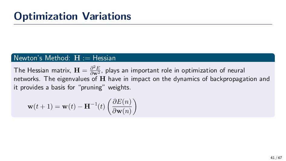
41. Optimization Variations Newton’s Method: H := Hessian The Hessian matrix, H = ∂2E ∂w2 , plays an important role in optimization of neural networks. The eigenvalues of H have in impact on the dynamics of backpropagation and it provides a basis for “pruning” weights. w(t + 1) = w(t) − H−1(t) ∂E(n) ∂w(n) 41 / 47
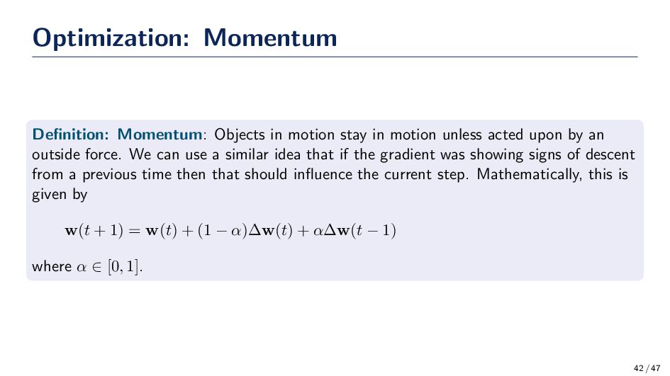
42. Optimization: Momentum Definition: Momentum: Objects in motion stay in motion unless acted upon by an outside force. We can use a similar idea that if the gradient was showing signs of descent from a previous time then that should influence the current step. Mathematically, this is given by w(t + 1) = w(t) + (1 − α)∆w(t) + α∆w(t − 1) where α ∈ [0, 1]. 42 / 47
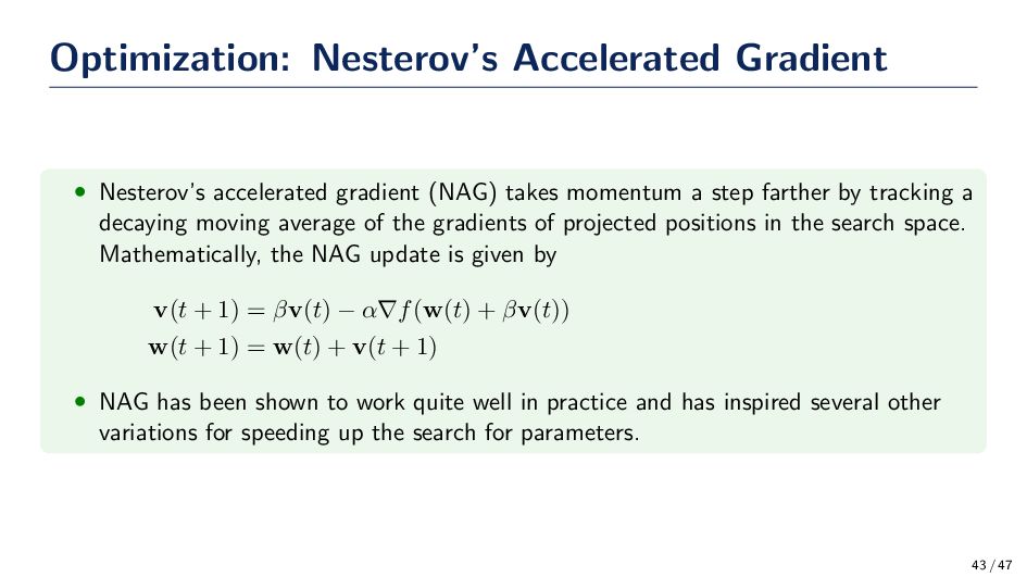
43. Optimization: Nesterov’s Accelerated Gradient • Nesterov’s accelerated gradient (NAG) takes momentum a step farther by tracking a decaying moving average of the gradients of projected positions in the search space. Mathematically, the NAG update is given by v(t + 1) = βv(t) − α∇f(w(t) + βv(t)) w(t + 1) = w(t) + v(t + 1) • NAG has been shown to work quite well in practice and has inspired several other variations for speeding up the search for parameters. 43 / 47
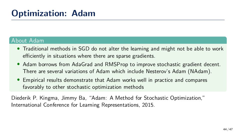
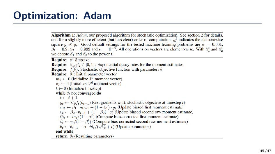
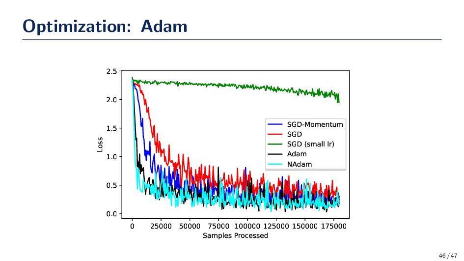
44. Optimization: Adam About Adam • Traditional methods in SGD do not alter the learning and might not be able to work efficiently in situations where there are sparse gradients. • Adam borrows from AdaGrad and RMSProp to improve stochastic gradient decent. There are several variations of Adam which include Nesterov’s Adam (NAdam). • Empirical results demonstrate that Adam works well in practice and compares favorably to other stochastic optimization methods Diederik P. Kingma, Jimmy Ba, “Adam: A Method for Stochastic Optimization,” International Conference for Learning Representations, 2015. 44 / 47
45. Optimization: Adam 45 / 47
46. Optimization: Adam 0 25000 50000 75000 100000 125000 150000 175000 Samples Processed 0.0 0.5 1.0 1.5 2.0 2.5 Loss SGD-Momentum SGD SGD (small lr) Adam NAdam 46 / 47
47. The End 47 / 47