can be difficult to achieve in practice, but learning a “weak” classifier is relatively easy • The weak learner is just a little bit better than a random guess. So for a two class problem the probability of error needs to be less than 0.5 • Constructing a weak learner is easy and low complexity. Think about it: getting a 99% on a Physics I exam is really difficult but getting a 51% is easy(ier)! • How can we generate and combine weak learners in a way that results in a strong classifier? • Adaboost was presented by Freund and Schapire and was the first practical boosting algorithm, and remains one of the most widely used and studied • Bias-Variance Dilemma: Adaboost reduces the bias and the variance of the model! 4 / 31
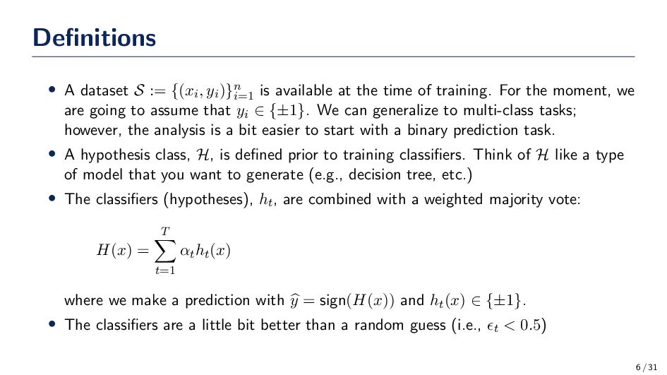
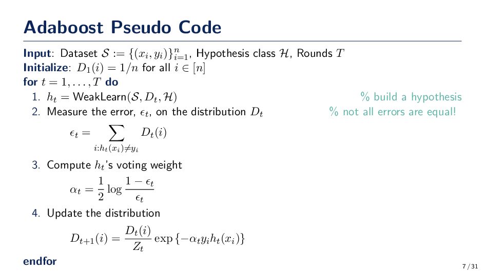
i=1 is available at the time of training. For the moment, we are going to assume that yi ∈ {±1}. We can generalize to multi-class tasks; however, the analysis is a bit easier to start with a binary prediction task. • A hypothesis class, H, is defined prior to training classifiers. Think of H like a type of model that you want to generate (e.g., decision tree, etc.) • The classifiers (hypotheses), ht, are combined with a weighted majority vote: H(x) = T t=1 αt ht (x) where we make a prediction with y = sign(H(x)) and ht (x) ∈ {±1}. • The classifiers are a little bit better than a random guess (i.e., ϵt < 0.5) 6 / 31
)}n i=1 , Hypothesis class H, Rounds T Initialize: D1 (i) = 1/n for all i ∈ [n] for t = 1, . . . , T do 1. ht = WeakLearn(S, Dt , H) % build a hypothesis 2. Measure the error, ϵt, on the distribution Dt % not all errors are equal! ϵt = i:ht(xi)̸=yi Dt (i) 3. Compute ht’s voting weight αt = 1 2 log 1 − ϵt ϵt 4. Update the distribution Dt+1 (i) = Dt (i) Zt exp {−αt yi ht (xi )} endfor 7 / 31
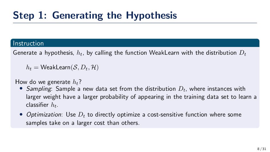
by calling the function WeakLearn with the distribution Dt ht = WeakLearn(S, Dt , H) How do we generate ht? • Sampling: Sample a new data set from the distribution Dt, where instances with larger weight have a larger probability of appearing in the training data set to learn a classifier ht. • Optimization: Use Dt to directly optimize a cost-sensitive function where some samples take on a larger cost than others. 8 / 31
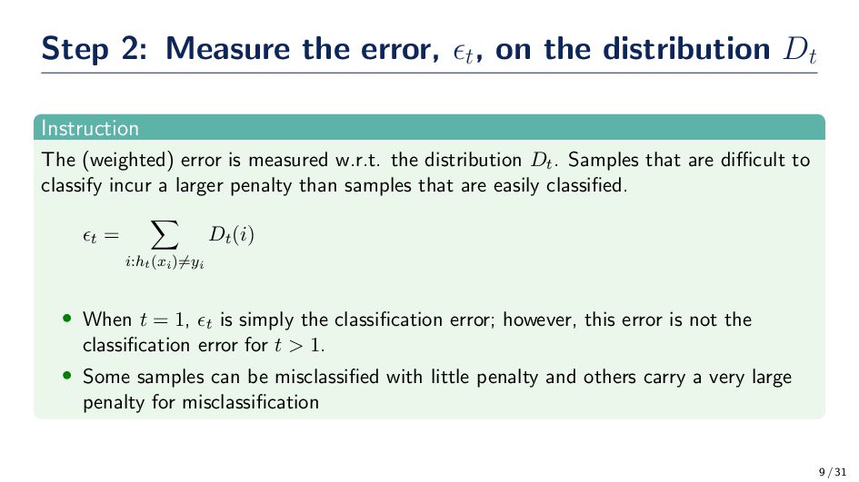
Dt Instruction The (weighted) error is measured w.r.t. the distribution Dt. Samples that are difficult to classify incur a larger penalty than samples that are easily classified. ϵt = i:ht(xi)̸=yi Dt (i) • When t = 1, ϵt is simply the classification error; however, this error is not the classification error for t > 1. • Some samples can be misclassified with little penalty and others carry a very large penalty for misclassification 9 / 31
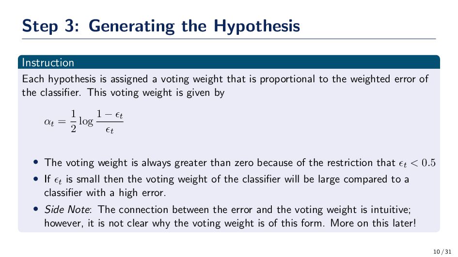
a voting weight that is proportional to the weighted error of the classifier. This voting weight is given by αt = 1 2 log 1 − ϵt ϵt • The voting weight is always greater than zero because of the restriction that ϵt < 0.5 • If ϵt is small then the voting weight of the classifier will be large compared to a classifier with a high error. • Side Note: The connection between the error and the voting weight is intuitive; however, it is not clear why the voting weight is of this form. More on this later! 10 / 31
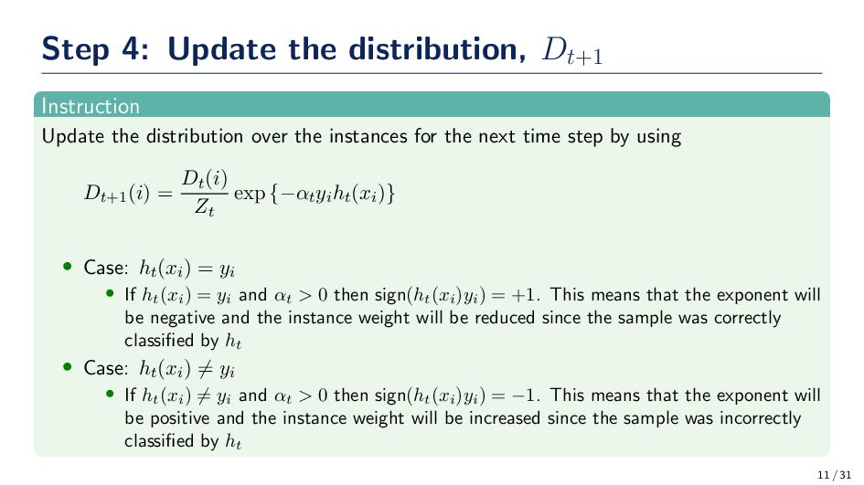
over the instances for the next time step by using Dt+1 (i) = Dt (i) Zt exp {−αt yi ht (xi )} • Case: ht (xi ) = yi • If ht (xi ) = yi and αt > 0 then sign(ht (xi )yi ) = +1. This means that the exponent will be negative and the instance weight will be reduced since the sample was correctly classified by ht • Case: ht (xi ) ̸= yi • If ht (xi ) ̸= yi and αt > 0 then sign(ht (xi )yi ) = −1. This means that the exponent will be positive and the instance weight will be increased since the sample was incorrectly classified by ht 11 / 31
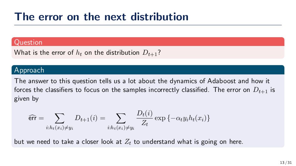
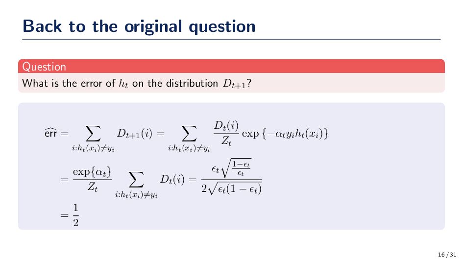
error of ht on the distribution Dt+1? Approach The answer to this question tells us a lot about the dynamics of Adaboost and how it forces the classifiers to focus on the samples incorrectly classified. The error on Dt+1 is given by err = i:ht(xi)̸=yi Dt+1 (i) = i:ht(xi)̸=yi Dt (i) Zt exp {−αt yi ht (xi )} but we need to take a closer look at Zt to understand what is going on here. 13 / 31
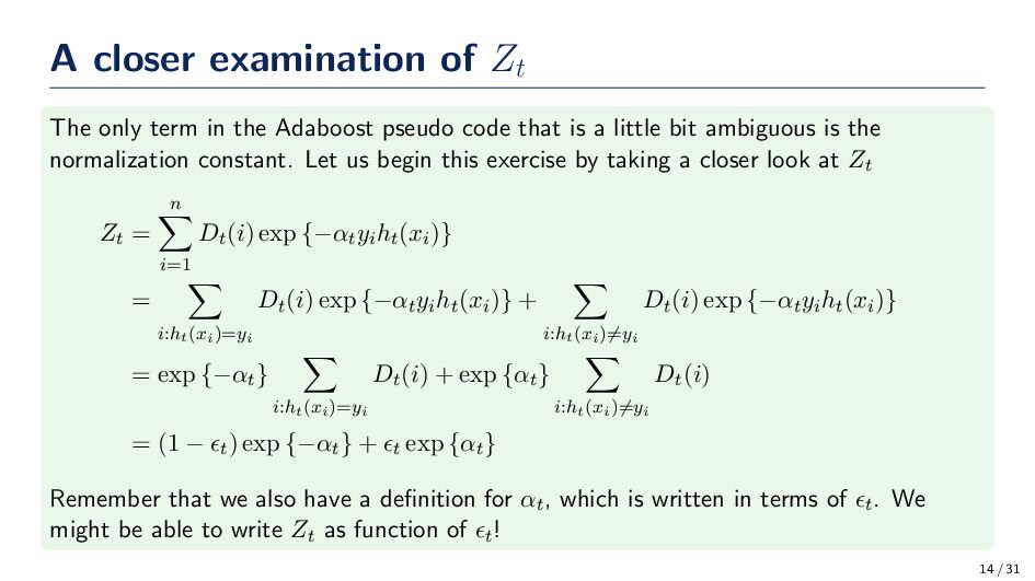
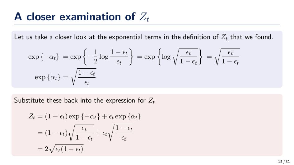
Adaboost pseudo code that is a little bit ambiguous is the normalization constant. Let us begin this exercise by taking a closer look at Zt Zt = n i=1 Dt (i) exp {−αt yi ht (xi )} = i:ht(xi)=yi Dt (i) exp {−αt yi ht (xi )} + i:ht(xi)̸=yi Dt (i) exp {−αt yi ht (xi )} = exp {−αt} i:ht(xi)=yi Dt (i) + exp {αt} i:ht(xi)̸=yi Dt (i) = (1 − ϵt ) exp {−αt} + ϵt exp {αt} Remember that we also have a definition for αt, which is written in terms of ϵt. We might be able to write Zt as function of ϵt! 14 / 31
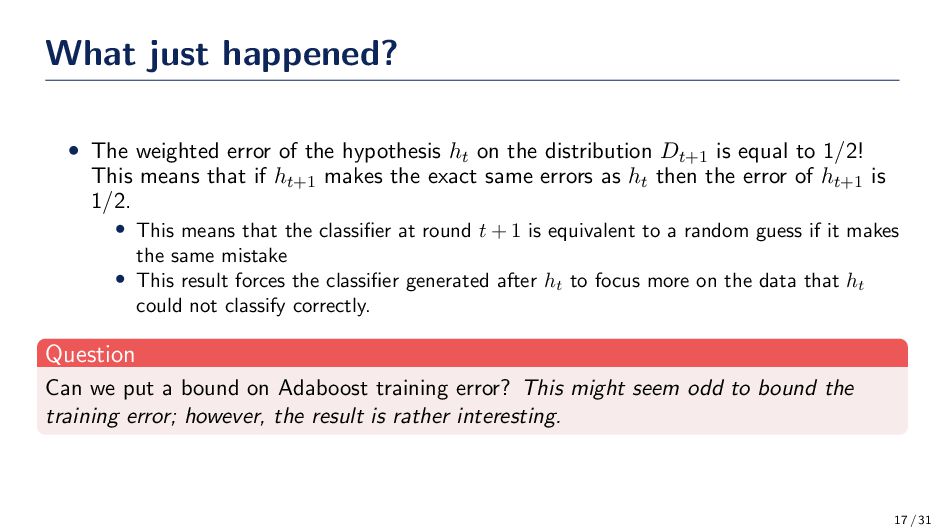
ht on the distribution Dt+1 is equal to 1/2! This means that if ht+1 makes the exact same errors as ht then the error of ht+1 is 1/2. • This means that the classifier at round t + 1 is equivalent to a random guess if it makes the same mistake • This result forces the classifier generated after ht to focus more on the data that ht could not classify correctly. Question Can we put a bound on Adaboost training error? This might seem odd to bound the training error; however, the result is rather interesting. 17 / 31
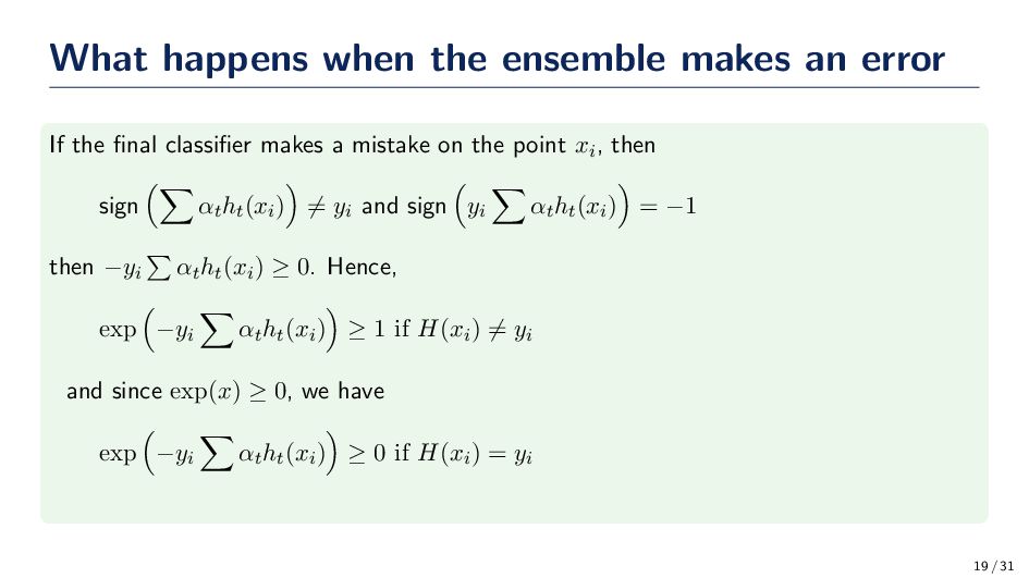
final classifier makes a mistake on the point xi, then sign αt ht (xi ) ̸= yi and sign yi αt ht (xi ) = −1 then −yi αt ht (xi ) ≥ 0. Hence, exp −yi αt ht (xi ) ≥ 1 if H(xi ) ̸= yi and since exp(x) ≥ 0, we have exp −yi αt ht (xi ) ≥ 0 if H(xi ) = yi 19 / 31
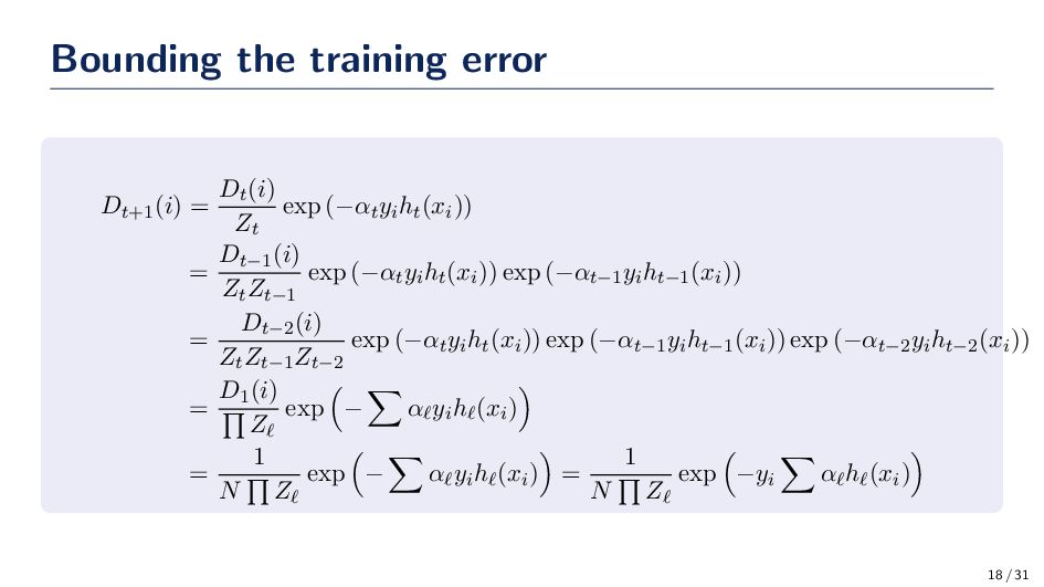
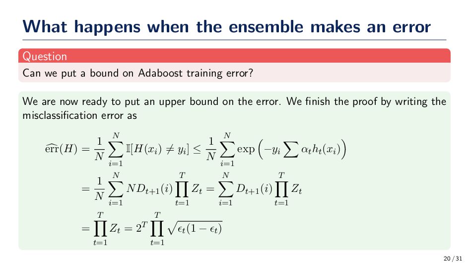
we put a bound on Adaboost training error? We are now ready to put an upper bound on the error. We finish the proof by writing the misclassification error as err(H) = 1 N N i=1 I[H(xi ) ̸= yi ] ≤ 1 N N i=1 exp −yi αt ht (xi ) = 1 N N i=1 NDt+1 (i) T t=1 Zt = N i=1 Dt+1 (i) T t=1 Zt = T t=1 Zt = 2T T t=1 ϵt (1 − ϵt ) 20 / 31
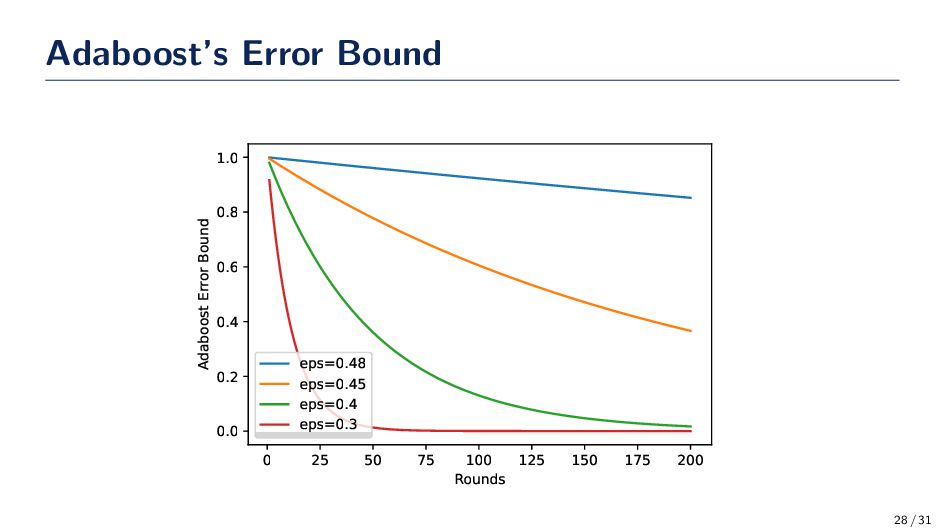
of Adaboost drops off exponentially as the number of hypotheses are added to the ensemble! This is a remarkable result • At first glance it would appear that this result would make us think that Adaboost is susceptible to overtraining; however, this is – generally – not the case. • Adaboost is actually surprisingly robust to overtraining! • The dynamics of Adaboost can be related to a game being played between the learner and the distribution. • Is there a relationship between the boosting algorithm and margin theory? Yup! • Adaboost is an incredibly simple algorithm that is backed by a lot of elegant theory. 21 / 31
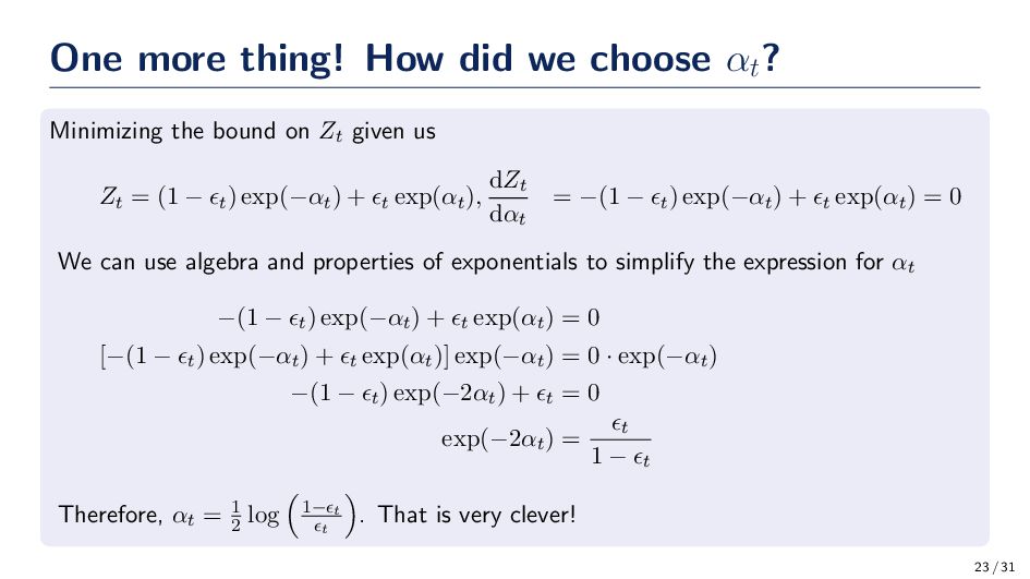
Why did we choose αt the way that we did? Recall that the training error is upper bounded by a product of Zt, so why don’t we minimize the upper bound? 22 / 31
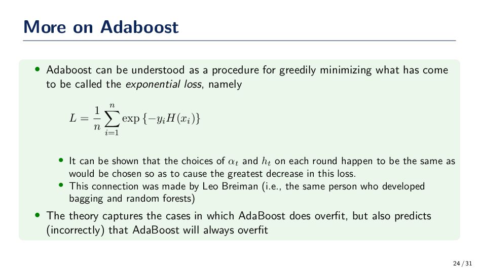
procedure for greedily minimizing what has come to be called the exponential loss, namely L = 1 n n i=1 exp {−yi H(xi )} • It can be shown that the choices of αt and ht on each round happen to be the same as would be chosen so as to cause the greatest decrease in this loss. • This connection was made by Leo Breiman (i.e., the same person who developed bagging and random forests) • The theory captures the cases in which AdaBoost does overfit, but also predicts (incorrectly) that AdaBoost will always overfit 24 / 31
6 x 4 2 0 2 4 6 8 y Decision Boundary Class A Class B 0.6 0.4 0.2 0.0 0.2 0.4 Score 0 20 40 60 80 100 120 140 160 Samples Decision Scores Class A Class B 27 / 31
weak learning models and combines them into a strong hypothesis. Adaboost has been shown to be very robust to overtraining. • There are a bunch of references available to learn more about the theory of Adaboost. • The version of Adaboost that we discussed in this lecture is known as Adaboost.M1, which is for binary prediction tasks. • Adaboost.M2 is for multiclass tasks, and there are many other variations of Adaboost too! 29 / 31
York, NY: Springer 1st edition. Robert E. Shapire and Yoav Freund (2012) Boosting: Foundations and Algorithms Cambridge, MA: MIT Press 1st edition. 30 / 31
![Machine Learning Lectures Adaboost Gregory Ditzler [email protected] February 24, 2024](https://files.speakerdeck.com/presentations/96d49c92267b4f08be1b58ae6544b7cf/slide_0.jpg)