University Ecological and Evolutionary Signal Processing & Informatics Lab Department of Electrical & Computer Engineering Philadelphia, PA, USA [email protected] http://gregoryditzler.com December 3, 2013
“Regardless of how complex the circuit becomes the analysis will always comeback to three main laws: Ohm’s law, Kirchoff’s current law, and Kirchoff’s voltage law.” –Me “All of the probabilistic inference in this book, no matter how complex, amount to repeated manipulations of the sum and product rule in probability theory” Christopher Bishop, PRML
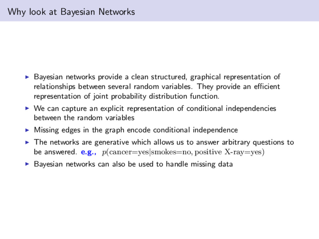
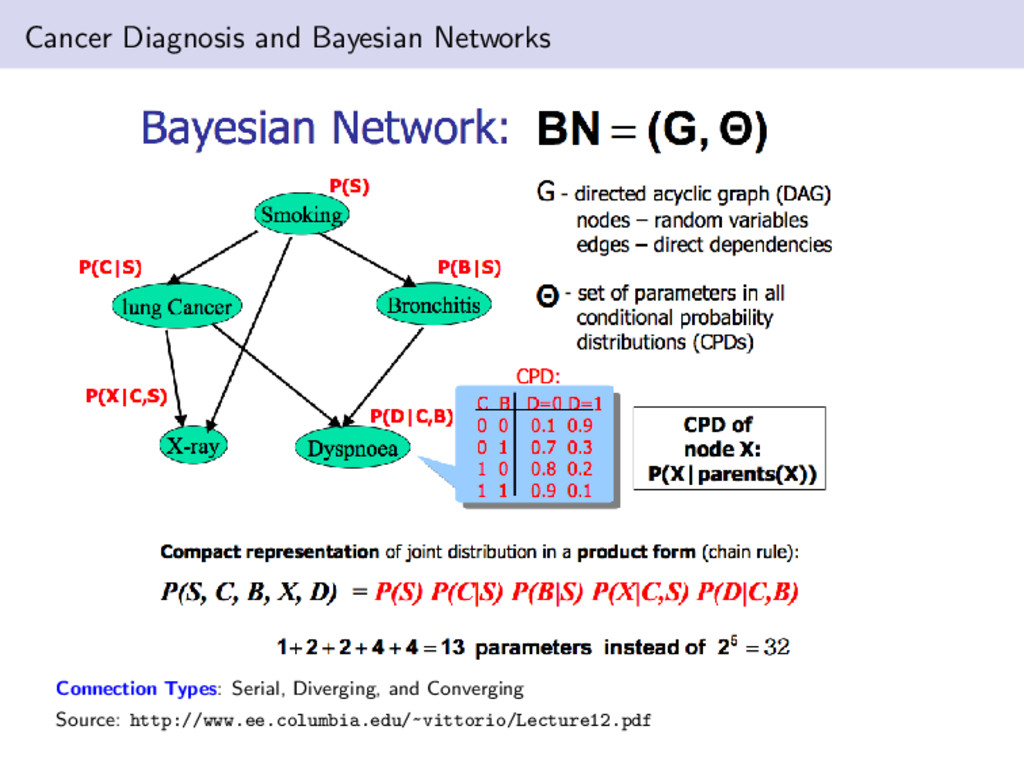
structured, graphical representation of relationships between several random variables. They provide an efficient representation of joint probability distribution function. We can capture an explicit representation of conditional independencies between the random variables Missing edges in the graph encode conditional independence The networks are generative which allows us to answer arbitrary questions to be answered. e.g., p(cancer=yes|smokes=no, positive X-ray=yes) Bayesian networks can also be used to handle missing data
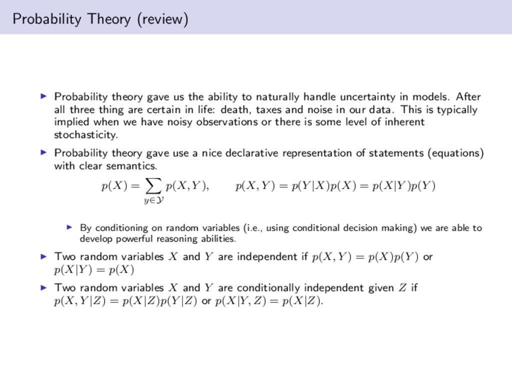
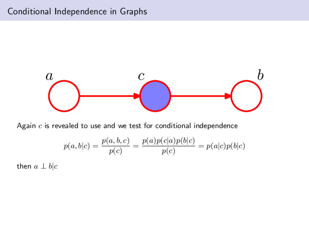
naturally handle uncertainty in models. After all three thing are certain in life: death, taxes and noise in our data. This is typically implied when we have noisy observations or there is some level of inherent stochasticity. Probability theory gave use a nice declarative representation of statements (equations) with clear semantics. p(X) = y∈Y p(X, Y ), p(X, Y ) = p(Y |X)p(X) = p(X|Y )p(Y ) By conditioning on random variables (i.e., using conditional decision making) we are able to develop powerful reasoning abilities. Two random variables X and Y are independent if p(X, Y ) = p(X)p(Y ) or p(X|Y ) = p(X) Two random variables X and Y are conditionally independent given Z if p(X, Y |Z) = p(X|Z)p(Y |Z) or p(X|Y, Z) = p(X|Z).
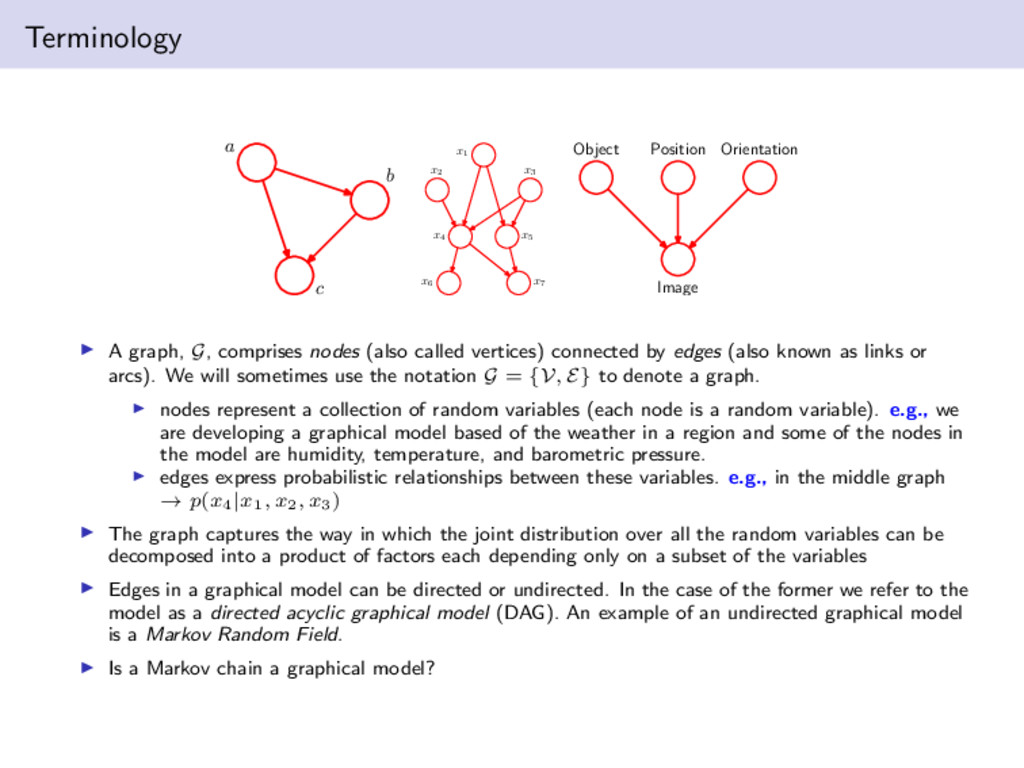
x7 Image Object Orientation Position A graph, G, comprises nodes (also called vertices) connected by edges (also known as links or arcs). We will sometimes use the notation G = {V, E} to denote a graph. nodes represent a collection of random variables (each node is a random variable). e.g., we are developing a graphical model based of the weather in a region and some of the nodes in the model are humidity, temperature, and barometric pressure. edges express probabilistic relationships between these variables. e.g., in the middle graph → p(x4|x1, x2, x3) The graph captures the way in which the joint distribution over all the random variables can be decomposed into a product of factors each depending only on a subset of the variables Edges in a graphical model can be directed or undirected. In the case of the former we refer to the model as a directed acyclic graphical model (DAG). An example of an undirected graphical model is a Markov Random Field. Is a Markov chain a graphical model?
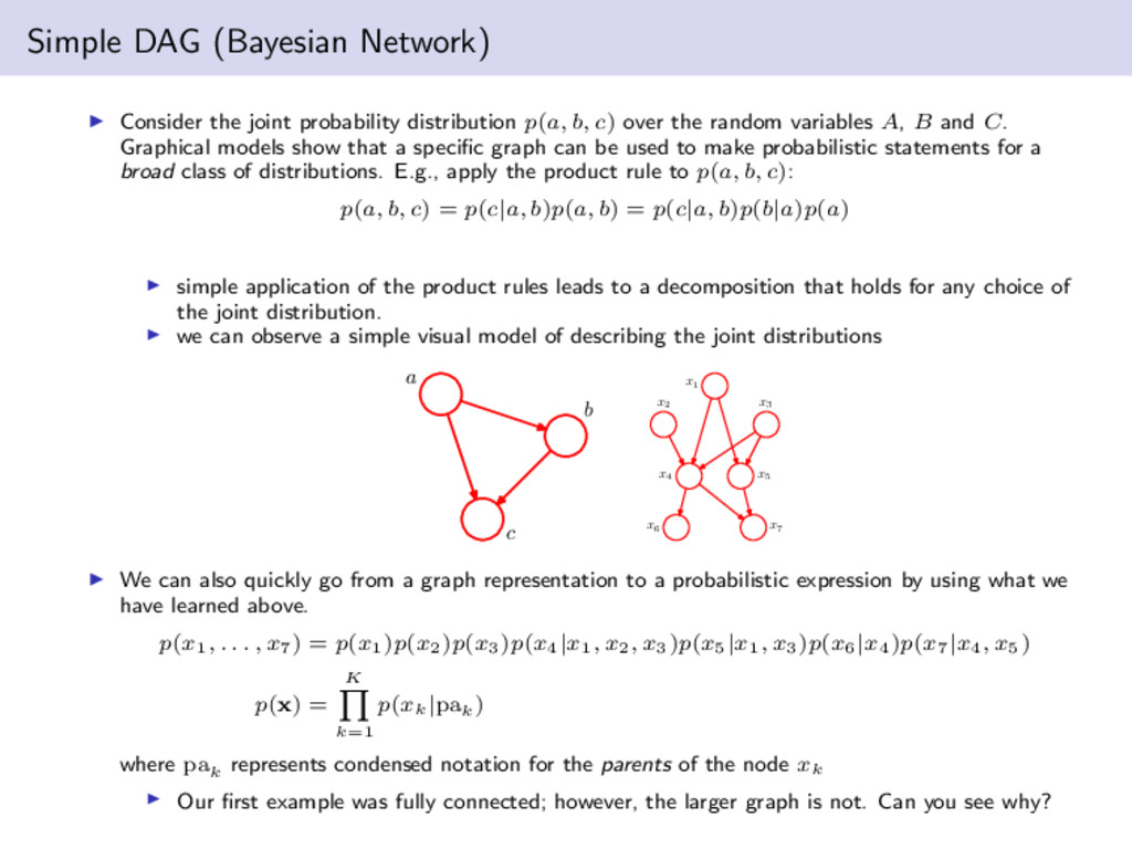
b, c) over the random variables A, B and C. Graphical models show that a specific graph can be used to make probabilistic statements for a broad class of distributions. E.g., apply the product rule to p(a, b, c): p(a, b, c) = p(c|a, b)p(a, b) = p(c|a, b)p(b|a)p(a) simple application of the product rules leads to a decomposition that holds for any choice of the joint distribution. we can observe a simple visual model of describing the joint distributions a b c x1 x2 x3 x4 x5 x6 x7 We can also quickly go from a graph representation to a probabilistic expression by using what we have learned above. p(x1, . . . , x7) = p(x1)p(x2)p(x3)p(x4|x1, x2, x3)p(x5|x1, x3)p(x6|x4)p(x7|x4, x5) p(x) = K k=1 p(xk|pak ) where pak represents condensed notation for the parents of the node xk Our first example was fully connected; however, the larger graph is not. Can you see why?
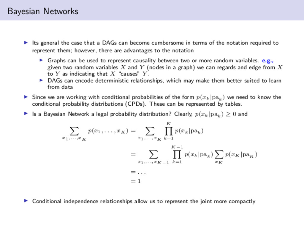
become cumbersome in terms of the notation required to represent them; however, there are advantages to the notation Graphs can be used to represent causality between two or more random variables. e.g., given two random variables X and Y (nodes in a graph) we can regards and edge from X to Y as indicating that X “causes” Y . DAGs can encode deterministic relationships, which may make them better suited to learn from data Since we are working with conditional probabilities of the form p(xk|pak ) we need to know the conditional probability distributions (CPDs). These can be represented by tables. Is a Bayesian Network a legal probability distribution? Clearly, p(xk|pak ) ≥ 0 and x1,...,xK p(x1, . . . , xK ) = x1,...,xK K k=1 p(xk|pak ) = x1,...,xK−1 K−1 k=1 p(xk|pak ) xK p(xK |paK ) = . . . = 1 Conditional independence relationships allow us to represent the joint more compactly
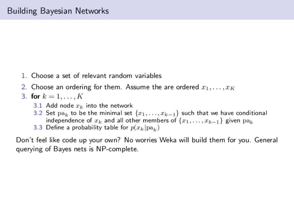
variables 2. Choose an ordering for them. Assume the are ordered x1 , . . . , xK 3. for k = 1, . . . , K 3.1 Add node xk into the network 3.2 Set pak to be the minimal set {x1, . . . , xk−1} such that we have conditional independence of xk and all other members of {x1, . . . , xk−1} given pak 3.3 Define a probability table for p(xk|pak ) Don’t feel like code up your own? No worries Weka will build them for you. General querying of Bayes nets is NP-complete.
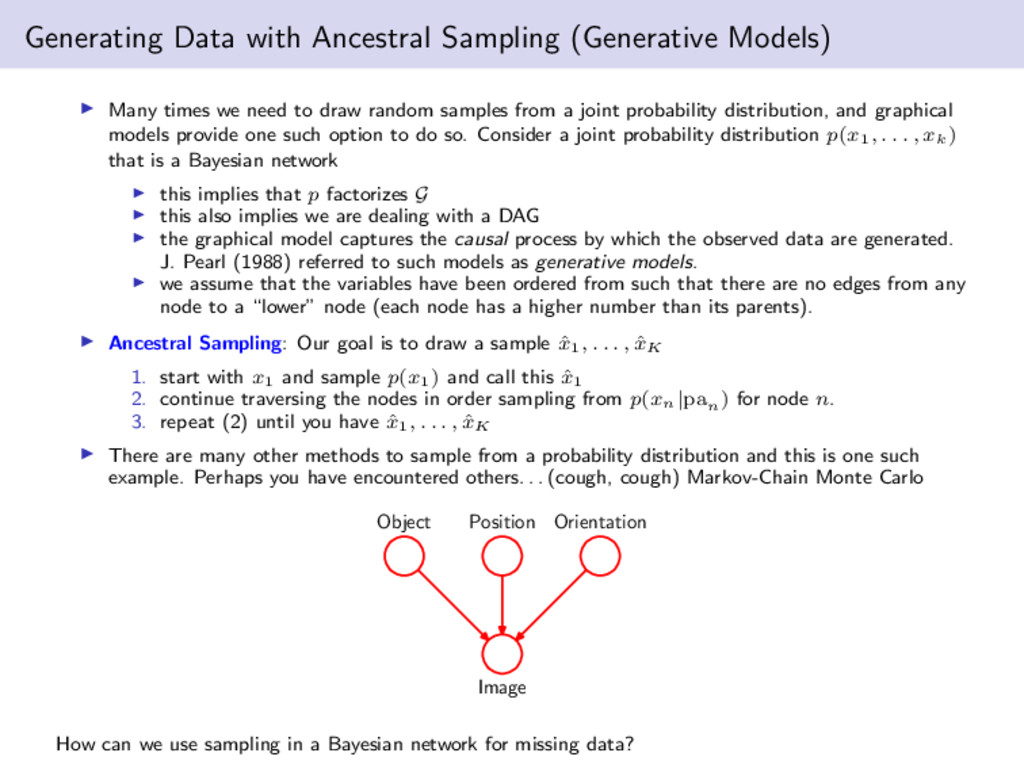
need to draw random samples from a joint probability distribution, and graphical models provide one such option to do so. Consider a joint probability distribution p(x1, . . . , xk) that is a Bayesian network this implies that p factorizes G this also implies we are dealing with a DAG the graphical model captures the causal process by which the observed data are generated. J. Pearl (1988) referred to such models as generative models. we assume that the variables have been ordered from such that there are no edges from any node to a “lower” node (each node has a higher number than its parents). Ancestral Sampling: Our goal is to draw a sample ˆ x1, . . . , ˆ xK 1. start with x1 and sample p(x1) and call this ˆ x1 2. continue traversing the nodes in order sampling from p(xn|pan ) for node n. 3. repeat (2) until you have ˆ x1, . . . , ˆ xK There are many other methods to sample from a probability distribution and this is one such example. Perhaps you have encountered others. . . (cough, cough) Markov-Chain Monte Carlo Image Object Orientation Position How can we use sampling in a Bayesian network for missing data?
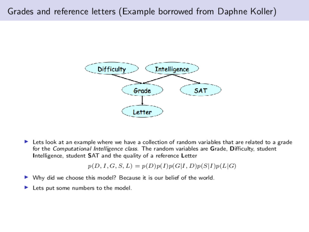
look at an example where we have a collection of random variables that are related to a grade for the Computational Intelligence class. The random variables are Grade, Difficulty, student Intelligence, student SAT and the quality of a reference Letter p(D, I, G, S, L) = p(D)p(I)p(G|I, D)p(S|I)p(L|G) Why did we choose this model? Because it is our belief of the world. Lets put some numbers to the model.
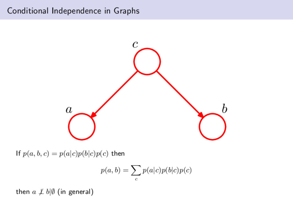
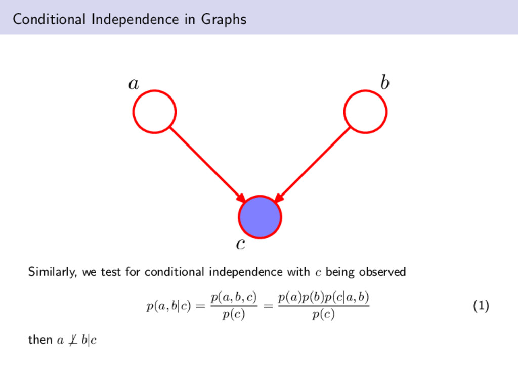
at the exactly the opposite of the first example. We now have p(a, b, c) = p(a)p(b)p(c|a, b) then marginalizing over c gives us p(a, b) = p(a)p(b). Hence a ⊥ b|∅
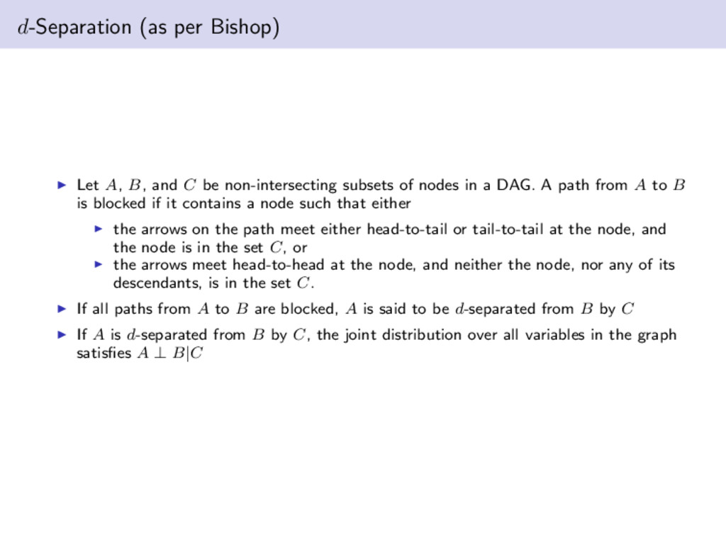
non-intersecting subsets of nodes in a DAG. A path from A to B is blocked if it contains a node such that either the arrows on the path meet either head-to-tail or tail-to-tail at the node, and the node is in the set C, or the arrows meet head-to-head at the node, and neither the node, nor any of its descendants, is in the set C. If all paths from A to B are blocked, A is said to be d-separated from B by C If A is d-separated from B by C, the joint distribution over all variables in the graph satisfies A ⊥ B|C