Upgrade to Pro — share decks privately, control downloads, hide ads and more …

[DTU PhD Summer School 2026] Tensor Networks fo...

Sponsored · Your Podcast. Everywhere. Effortlessly. Share. Educate. Inspire. Entertain. You do you. We'll handle the rest.
Avatar for Kazu Ghalamkari Kazu Ghalamkari
August 27, 2026
17

[DTU PhD Summer School 2026] Tensor Networks for Density Estimation Beyond KL Divergence

Slides used in Tensor Networks for Density Estimation Beyond KL Divergence
at PhD Summer School at DTU (2026), 02901 Advanced Topics in Machine Learning: Tensor Networks for Machine Learning
27th Aug. 2026, 1:00 pm – 4:00 pm @ Summer school in DTU (Lyngby campus)

How can we estimate the true distribution underlying observed data? This is a fundamental question in machine learning. In this lecture, I will show that tensor decomposition is particularly well suited to discrete (categorical) density estimation, because it can naturally exploit the discreteness of tensor indices. We will then discuss recent developments in tensor-based density estimation beyond the Kullback–Leibler (KL) divergence, with a focus on improving robustness to noise and outliers. Although the KL divergence is often easier to optimize than other divergences, it is known to be less robust to outliers and noise. To address this issue, we will see efficient closed-form optimization methods based on a doubly bounded EM algorithm, as well as a relaxation approach to density estimation that uses deformed algebra to flatten the feasible set, thereby enabling iterative convex optimization. We will also discuss the limitations of conventional low-rank modeling approaches and introduce tensor many-body decomposition as an alternative energy-based modeling for density estimation.

Exercise:
https://gist.github.com/gkazunii/38b1cba9f20541ddc589ca57e28af9b7

Quiz:
https://gist.github.com/gkazunii/38b1cba9f20541ddc589ca57e28af9b7#file-quiz-md

Whiteboard:
https://gkazu.info/wp-content/uploads/2026/08/whiteboard_note1.pdf

Avatar for Kazu Ghalamkari

Kazu Ghalamkari

August 27, 2026

More Decks by Kazu Ghalamkari

Transcript

  1. @KazuGhalamkari Tensor Networks for Density Estimation Beyond KL Divergence Kazu

    Ghalamkari @ Technical University of Denmark PhD summer school “02901 Advanced Topics in Machine Learning: Tensor Networks for Machine Learning”, DTU, 27th Aug. 2026
  2. @KazuGhalamkari Tensor Networks for Density Estimation Beyond KL Divergence Kazu

    Ghalamkari @ Technical University of Denmark PhD summer school “02901 Advanced Topics in Machine Learning: Tensor Networks for Machine Learning”, DTU, 27th Aug. 2026
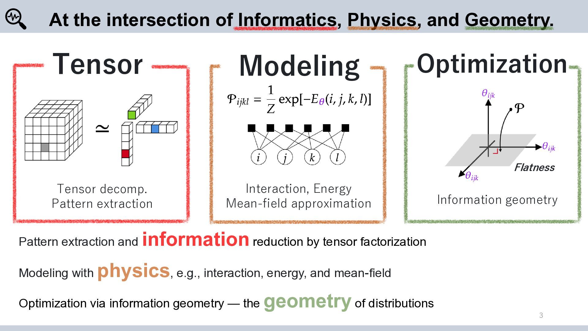
  3. At the intersection of Informatics, Physics, and Geometry. Tensor Modeling

    Optimization Flatness Tensor decomp. Pattern extraction Interaction, Energy Mean-field approximation Information geometry Pattern extraction and information reduction by tensor factorization Modeling with physics, e.g., interaction, energy, and mean-field Optimization via information geometry — the geometry of distributions 3
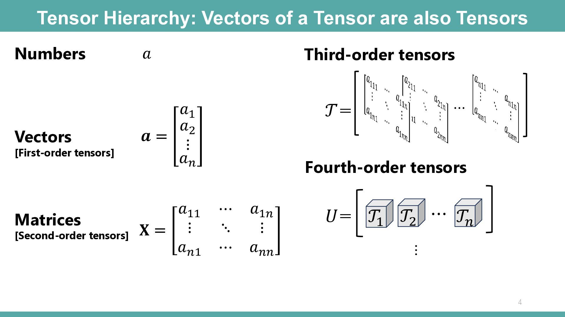
  4. Tensor Hierarchy: Vectors of a Tensor are also Tensors Numbers

    𝑎 Vectors 𝑎1 𝑎2 𝒂= ⋮ 𝑎𝑛 [First-order tensors] ⋯ 𝒯= Fourth-order tensors ⋯ ⋱ ⋯ 𝑎1𝑛 ⋮ 𝑎𝑛𝑛 𝑈= 𝒯1 𝒯2 ⋯ 𝒯𝑛 ⋯ 𝑎11 Matrices ⋮ [Second-order tensors] 𝐗 = 𝑎𝑛1 Third-order tensors 4
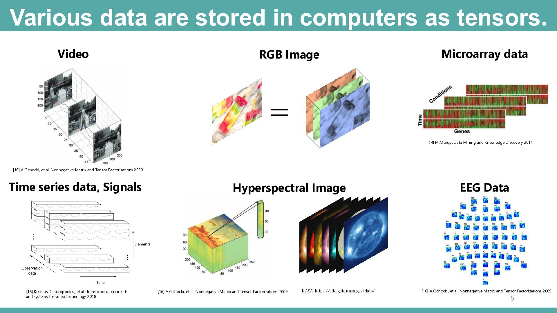
  5. Various data are stored in computers as tensors. Video RGB

    Image Microarray data = [14] M.Mørup, Data Mining and Knowledge Discovery 2011 [16] A.Cichocki, et al. Nonnegative Matrix and Tensor Factorizations 2009 Time series data, Signals [15] Kosmas Dimitropoulos, et al. Transactions on circuits and systems for video technology 2018 Hyperspectral Image [16] A.Cichocki, et al. Nonnegative Matrix and Tensor Factorizations 2009 NASA, https://sdo.gsfc.nasa.gov/data/ EEG Data [16] A.Cichocki, et al. Nonnegative Matrix and Tensor Factorizations 2009 5
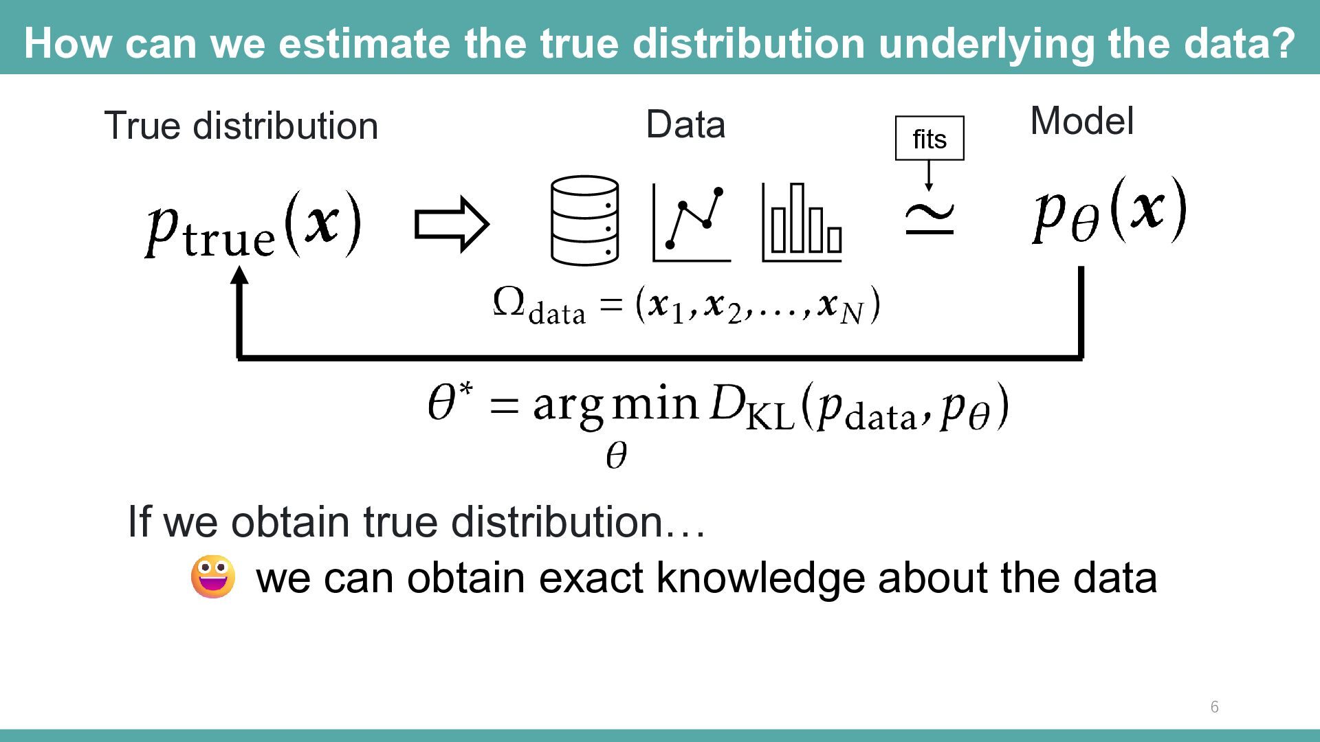
  6. How can we estimate the true distribution underlying the data?

    True distribution Data fits Model If we obtain true distribution… we can obtain exact knowledge about the data 6
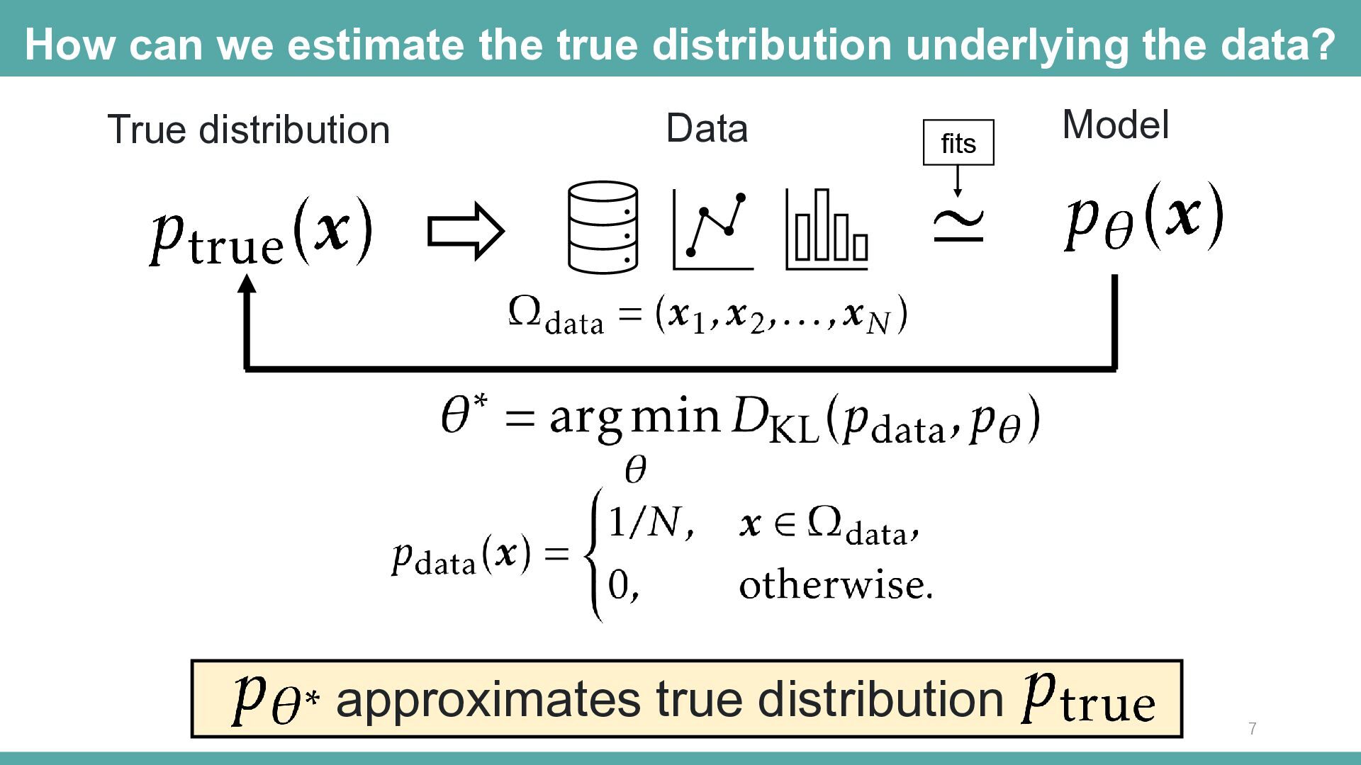
  7. How can we estimate the true distribution underlying the data?

    True distribution Data fits approximates true distribution Model 7
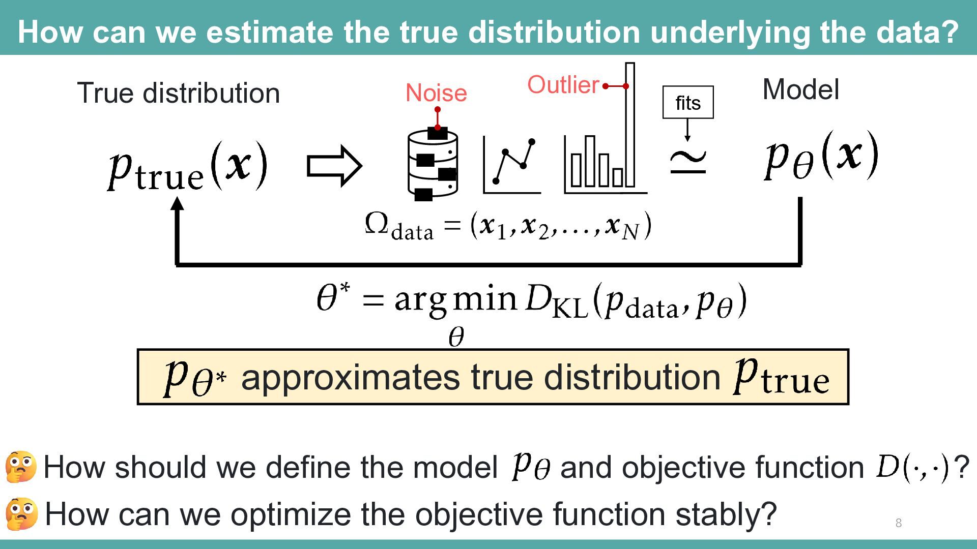
  8. How can we estimate the true distribution underlying the data?

    True distribution Noise Outlier fits Model approximates true distribution How should we define the model and objective function How can we optimize the objective function stably? ? 8
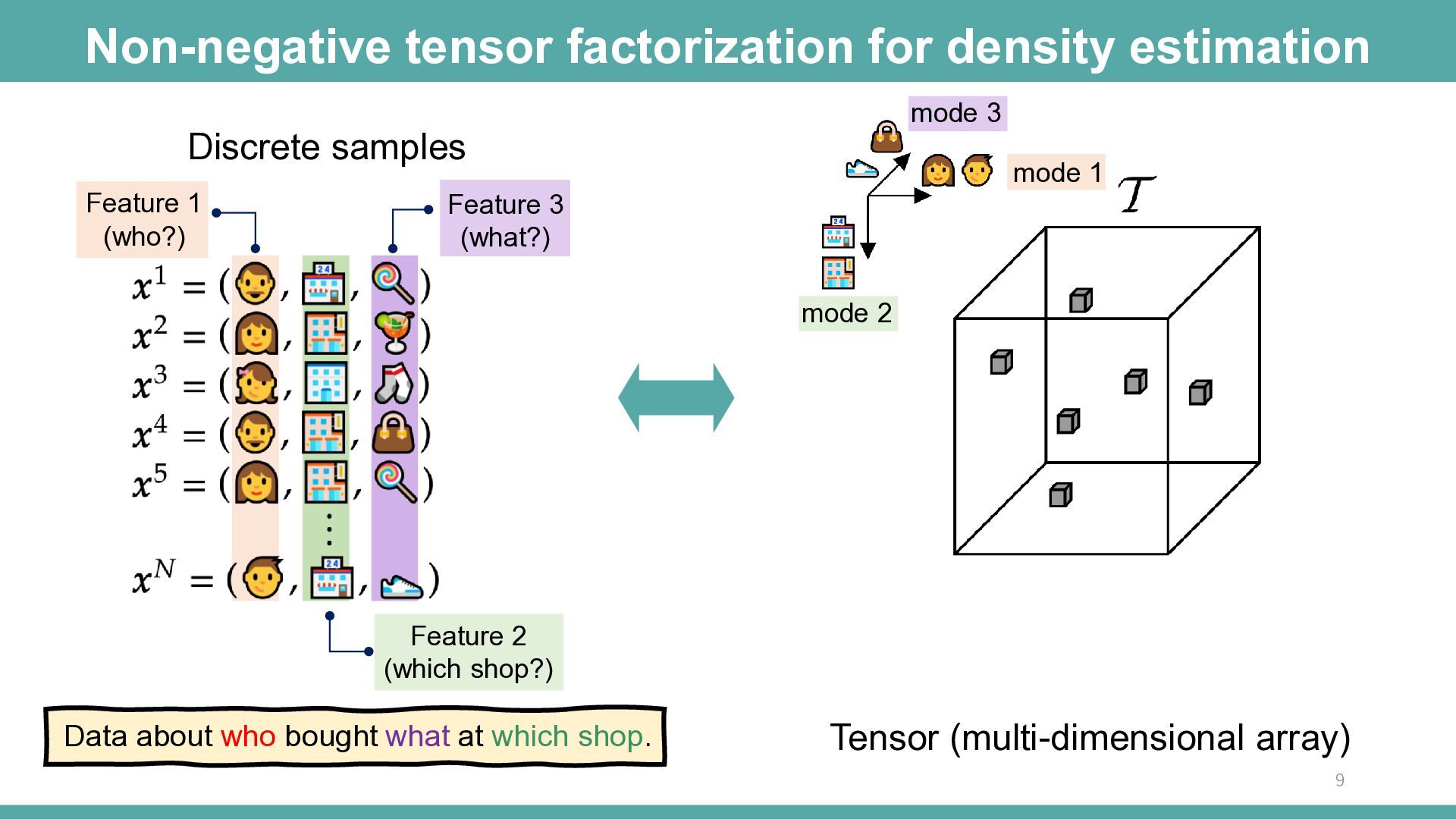
  9. Non-negative tensor factorization for density estimation mode 3 Discrete samples

    Feature 1 (who?) mode 1 Feature 3 (what?) mode 2 Feature 2 (which shop?) Data about who bought what at which shop. Tensor (multi-dimensional array) 9
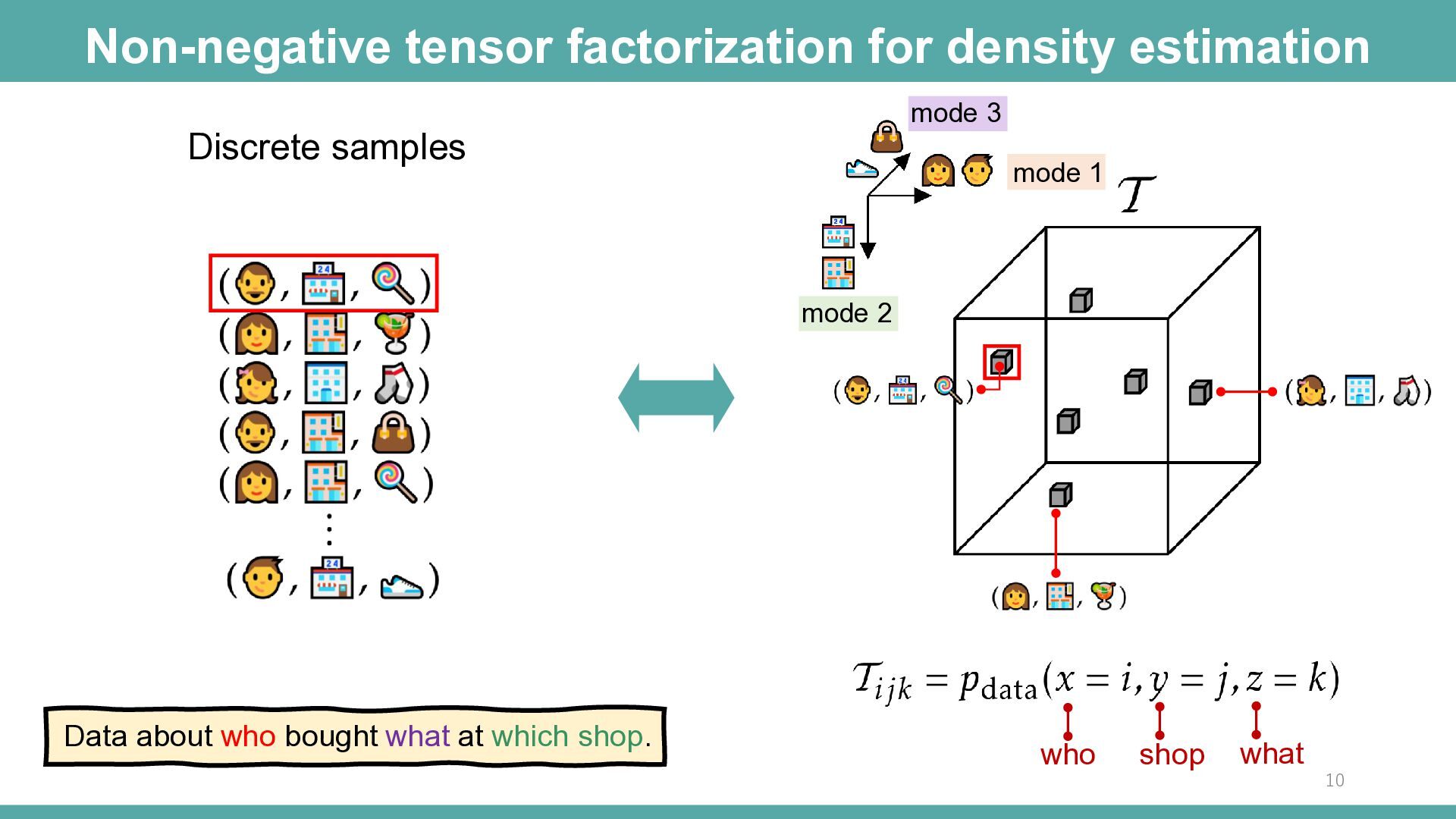
  10. Non-negative tensor factorization for density estimation mode 3 Discrete samples

    mode 1 mode 2 Data about who bought what at which shop. who shop what 10
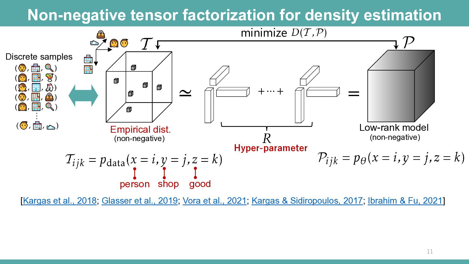
  11. Non-negative tensor factorization for density estimation minimize Discrete samples +⋯+

    = Low-rank model Empirical dist. (non-negative) (non-negative) Hyper-parameter person shop good [Kargas et al., 2018; Glasser et al., 2019; Vora et al., 2021; Kargas & Sidiropoulos, 2017; Ibrahim & Fu, 2021] 11
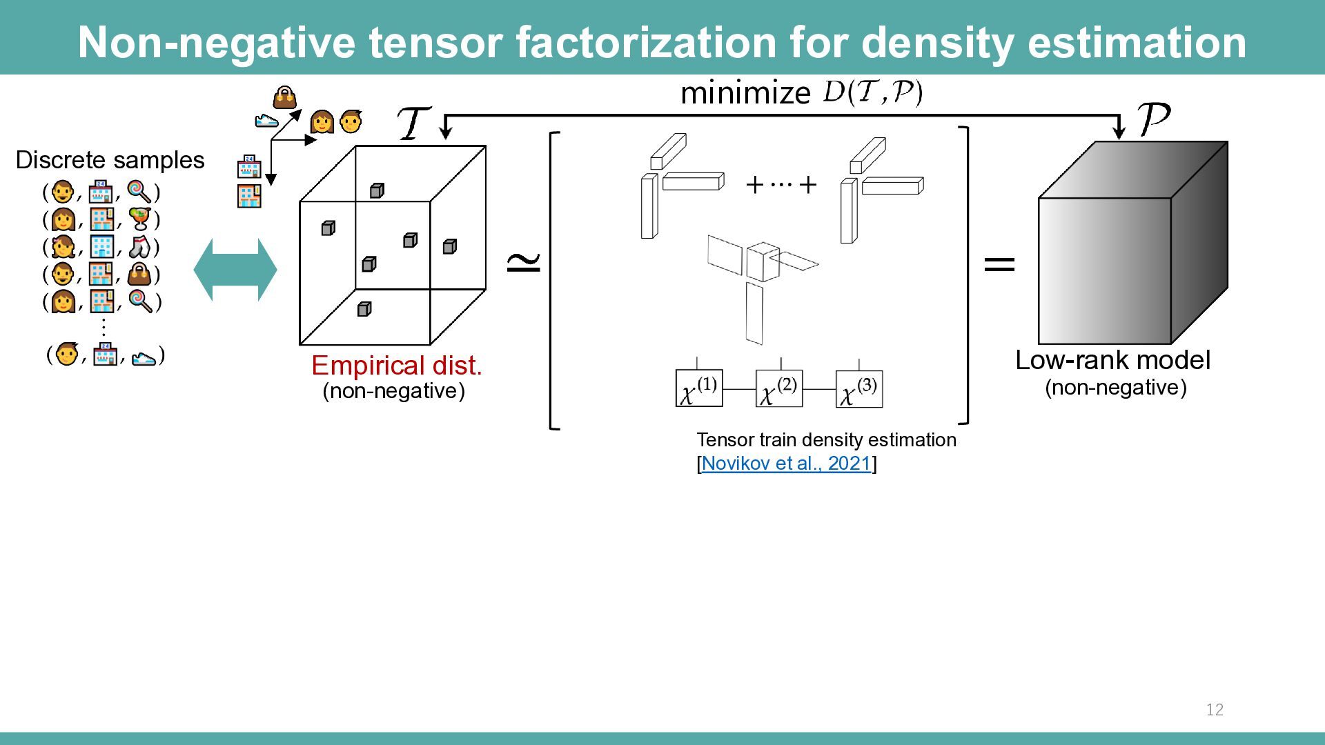
  12. Non-negative tensor factorization for density estimation minimize Discrete samples +⋯+

    = Low-rank model Empirical dist. (non-negative) (non-negative) Tensor train density estimation [Novikov et al., 2021] 12
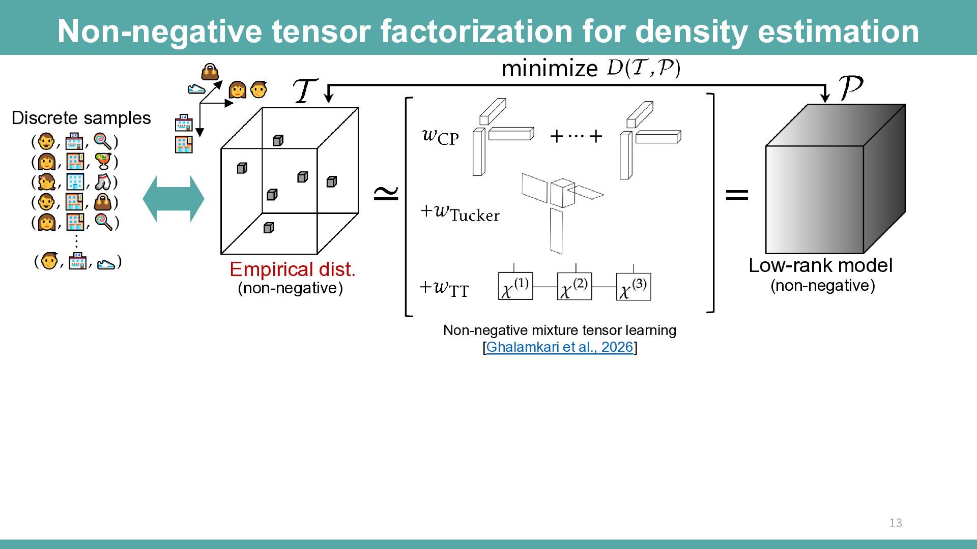
  13. Non-negative tensor factorization for density estimation minimize Discrete samples +⋯+

    = Low-rank model Empirical dist. (non-negative) (non-negative) Non-negative mixture tensor learning [Ghalamkari et al., 2026] 13
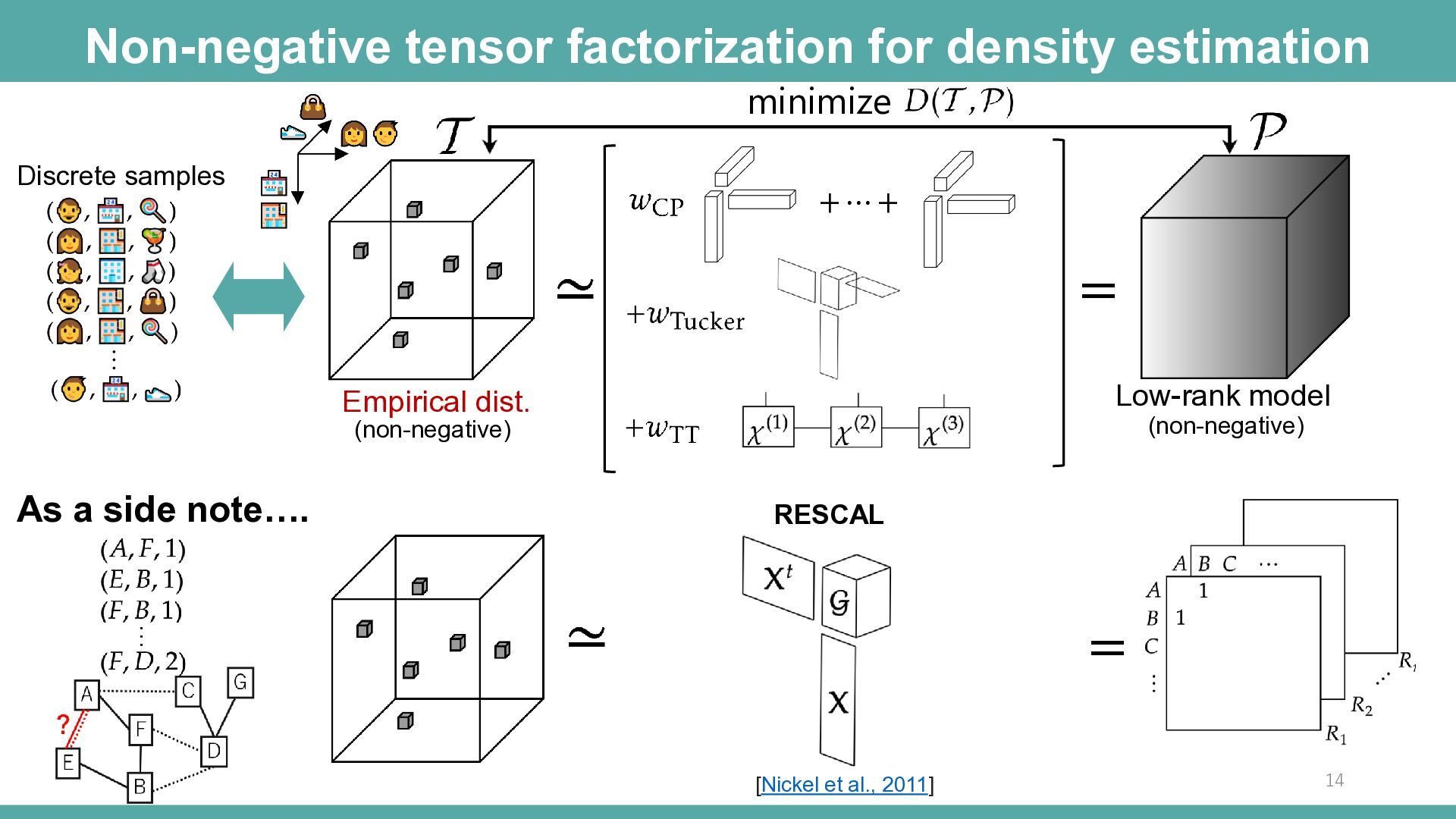
  14. Non-negative tensor factorization for density estimation minimize Discrete samples +⋯+

    = Low-rank model Empirical dist. (non-negative) (non-negative) As a side note…. RESCAL … = [Nickel et al., 2011] 14
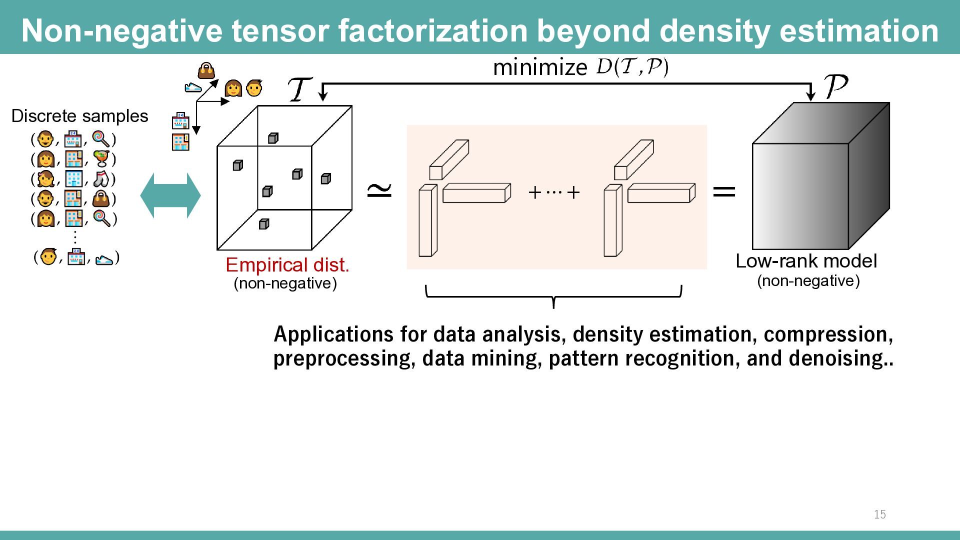
  15. Non-negative tensor factorization beyond density estimation minimize Discrete samples +⋯+

    Empirical dist. (non-negative) = Low-rank model (non-negative) Applications for data analysis, density estimation, compression, preprocessing, data mining, pattern recognition, and denoising.. 15
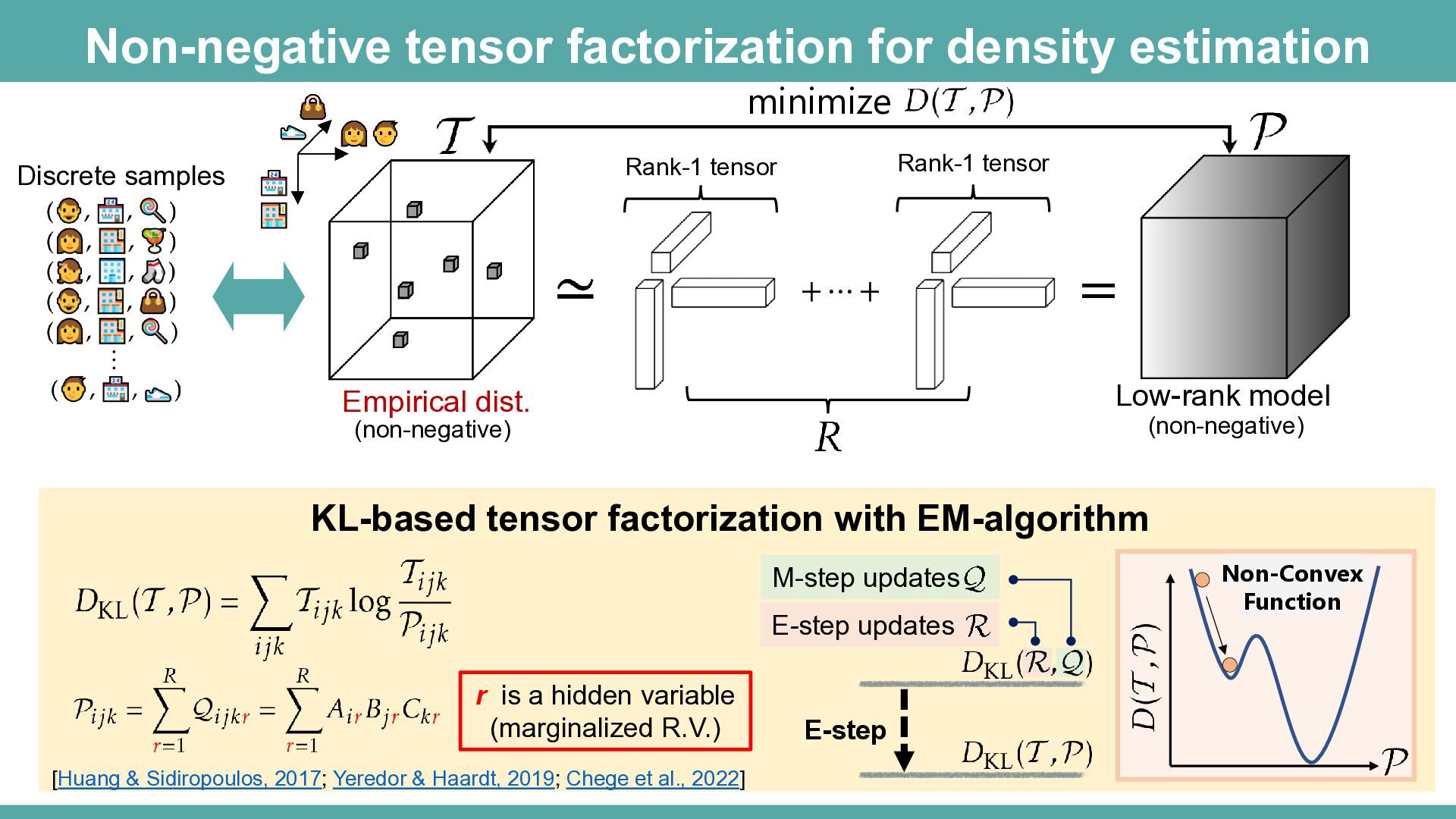
  16. Non-negative tensor factorization for density estimation minimize Rank-1 tensor Rank-1

    tensor Discrete samples +⋯+ = Low-rank model Empirical dist. (non-negative) (non-negative) KL-based tensor factorization with EM-algorithm M-step updates E-step updates r is a hidden variable (marginalized R.V.) [Huang & Sidiropoulos, 2017; Yeredor & Haardt, 2019; Chege et al., 2022] Non-Convex Function E-step 16
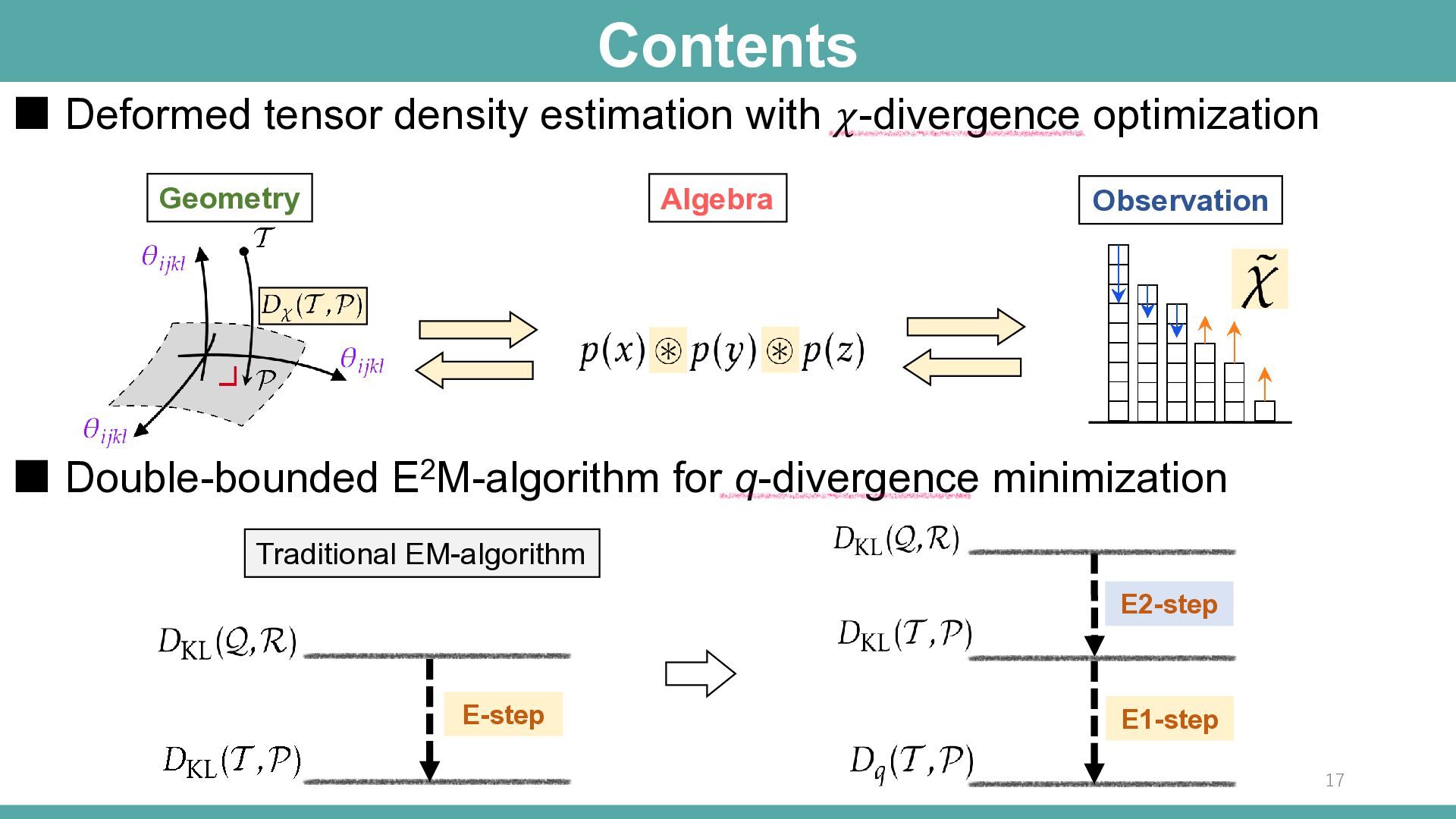
  17. Contents ▪ Deformed tensor density estimation with 𝜒-divergence optimization Geometry

    Algebra Observation ▪ Double-bounded E2M-algorithm for q-divergence minimization Traditional EM-algorithm E2-step E-step E1-step 17
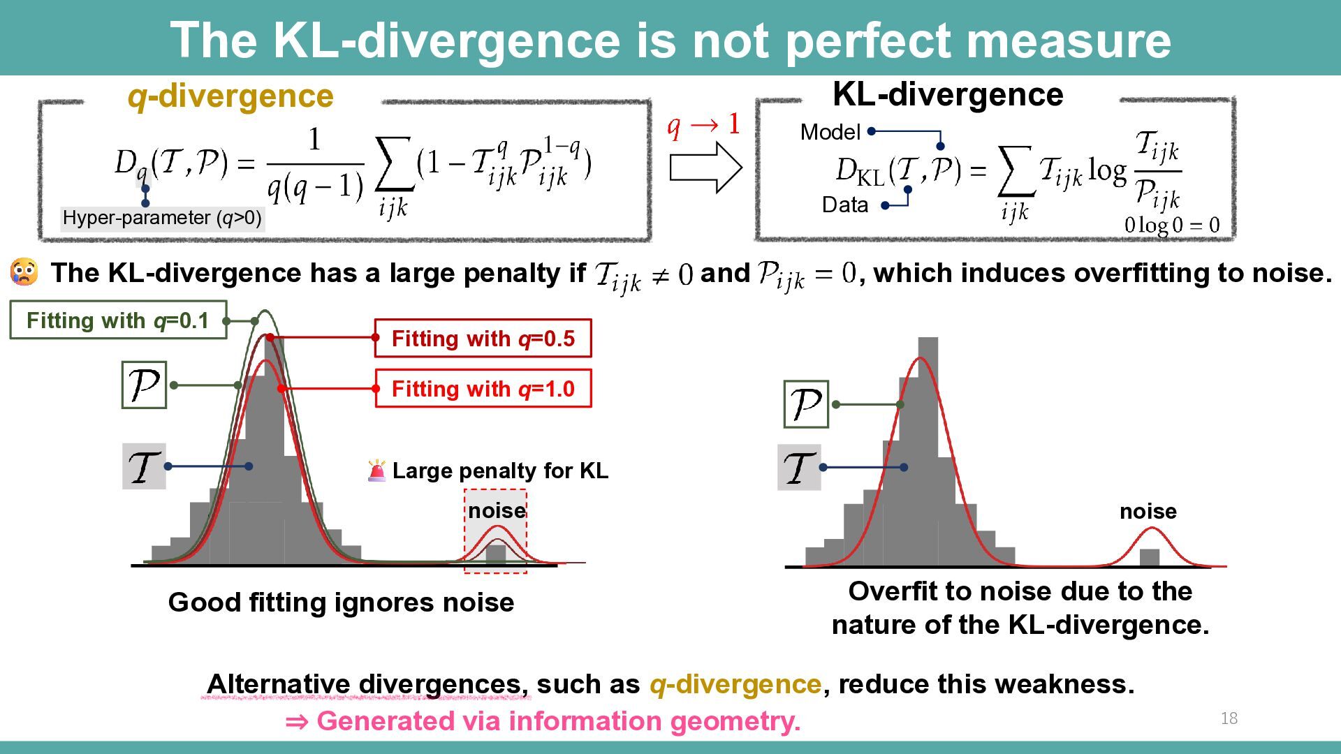
  18. The KL-divergence is not perfect measure KL-divergence q-divergence Model Data

    Hyper-parameter (q>0) The KL-divergence has a large penalty if Fitting with q=0.1 and , which induces overfitting to noise. Fitting with q=0.5 Fitting with q=1.0 Large penalty for KL noise Good fitting ignores noise noise Overfit to noise due to the nature of the KL-divergence. Alternative divergences, such as q-divergence, reduce this weakness. ⇒ Generated via information geometry. 18
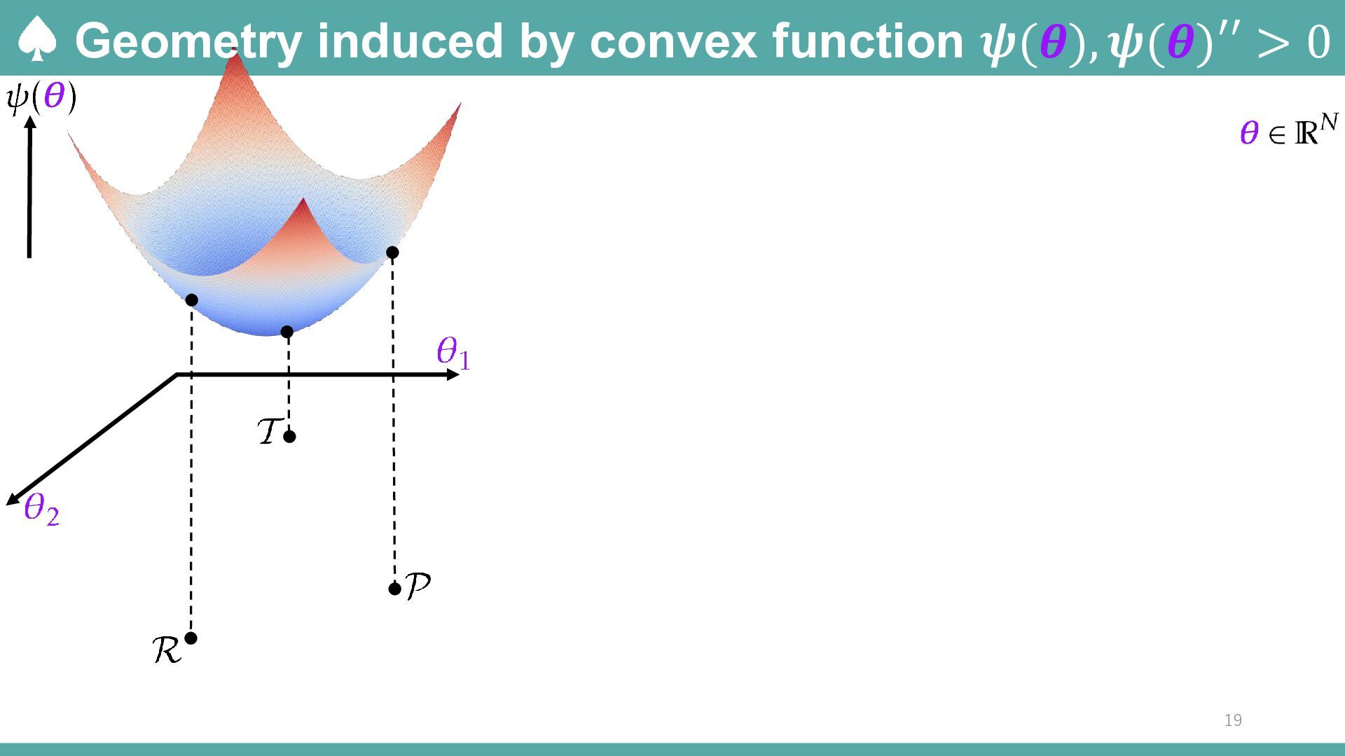
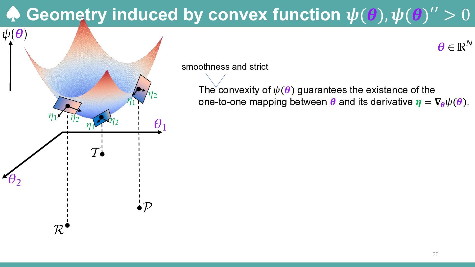
  19. Geometry induced by convex function 𝝍(𝜽), 𝝍(𝜽)′′ > 0 smoothness

    and strict The convexity of 𝜓(𝜽) guarantees the existence of the one-to-one mapping between 𝜽 and its derivative 𝜼 = 𝛁𝜽 𝜓(𝜽). 20
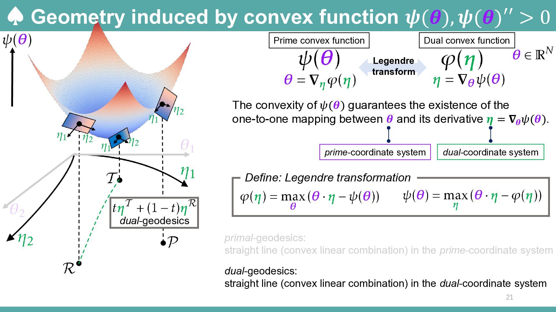
  20. Geometry induced by convex function 𝝍(𝜽), 𝝍(𝜽)′′ > 0 Dual

    convex function Prime convex function Legendre transform The convexity of 𝜓(𝜽) guarantees the existence of the one-to-one mapping between 𝜽 and its derivative 𝜼 = 𝛁𝜽 𝜓(𝜽). prime-coordinate system dual-coordinate system Define: Legendre transformation dual-geodesics primal-geodesics: straight line (convex linear combination) in the prime-coordinate system dual-geodesics: straight line (convex linear combination) in the dual-coordinate system 21
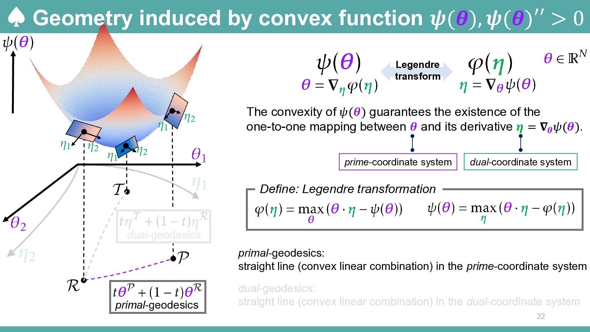
  21. Geometry induced by convex function 𝝍(𝜽), 𝝍(𝜽)′′ > 0 Legendre

    transform The convexity of 𝜓(𝜽) guarantees the existence of the one-to-one mapping between 𝜽 and its derivative 𝜼 = 𝛁𝜽 𝜓(𝜽). prime-coordinate system dual-coordinate system Define: Legendre transformation dual-geodesics primal-geodesics: straight line (convex linear combination) in the prime-coordinate system primal-geodesics dual-geodesics: straight line (convex linear combination) in the dual-coordinate system 22
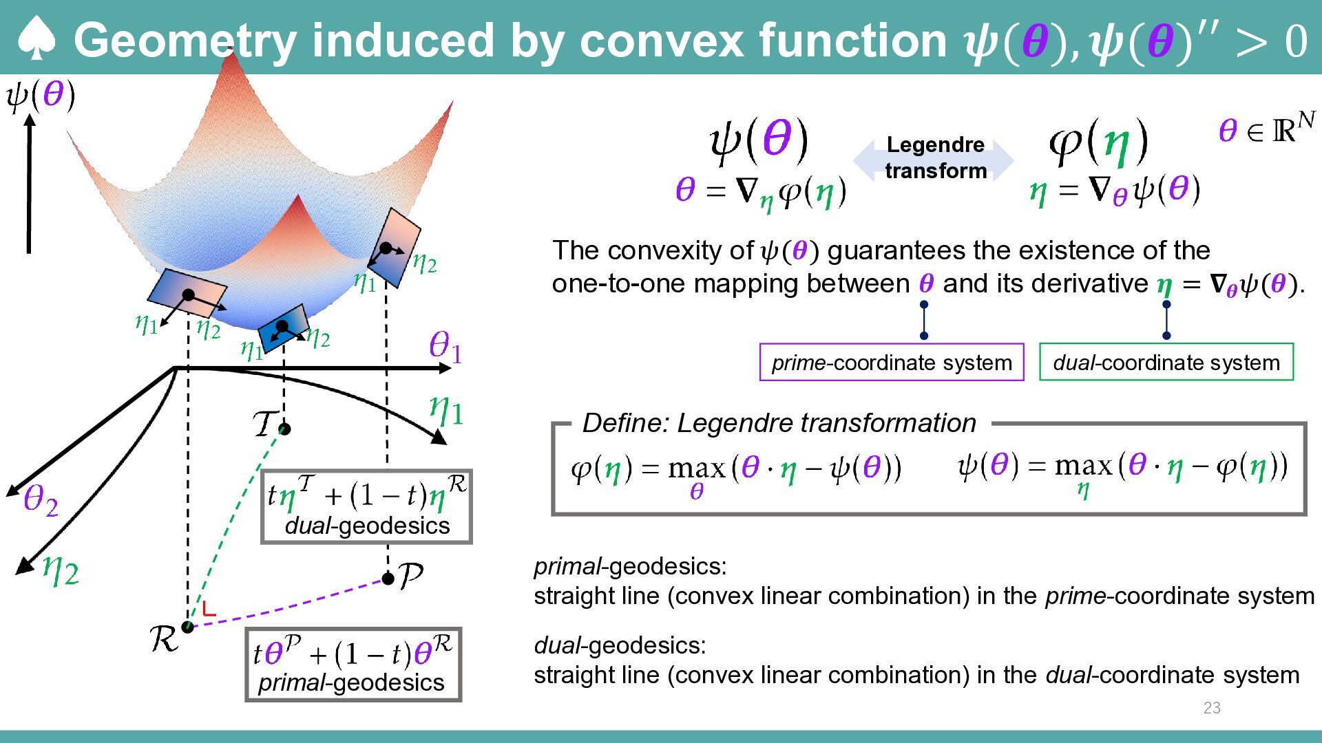
  22. Geometry induced by convex function 𝝍(𝜽), 𝝍(𝜽)′′ > 0 Legendre

    transform The convexity of 𝜓(𝜽) guarantees the existence of the one-to-one mapping between 𝜽 and its derivative 𝜼 = 𝛁𝜽 𝜓(𝜽). prime-coordinate system dual-coordinate system Define: Legendre transformation dual-geodesics primal-geodesics: straight line (convex linear combination) in the prime-coordinate system primal-geodesics dual-geodesics: straight line (convex linear combination) in the dual-coordinate system 23
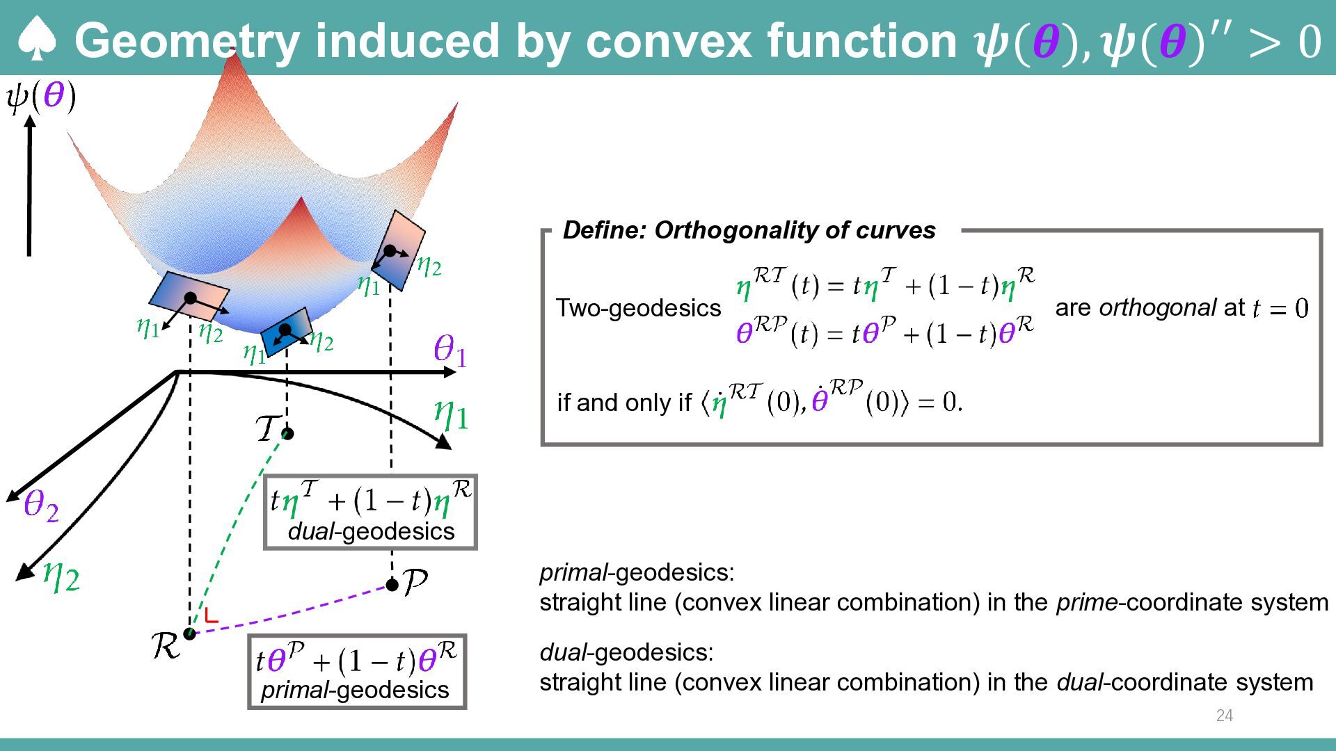
  23. Geometry induced by convex function 𝝍(𝜽), 𝝍(𝜽)′′ > 0 Define:

    Orthogonality of curves Two-geodesics are orthogonal at if and only if dual-geodesics primal-geodesics: straight line (convex linear combination) in the prime-coordinate system primal-geodesics dual-geodesics: straight line (convex linear combination) in the dual-coordinate system 24
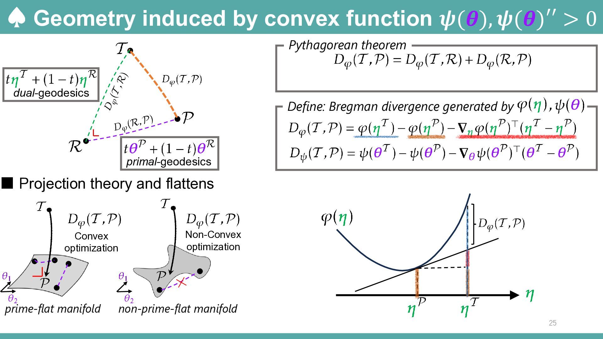
  24. Geometry induced by convex function 𝝍(𝜽), 𝝍(𝜽)′′ > 0 Pythagorean

    theorem dual-geodesics Define: Bregman divergence generated by primal-geodesics ▪ Projection theory and flattens Convex optimization prime-flat manifold Non-Convex optimization non-prime-flat manifold 25
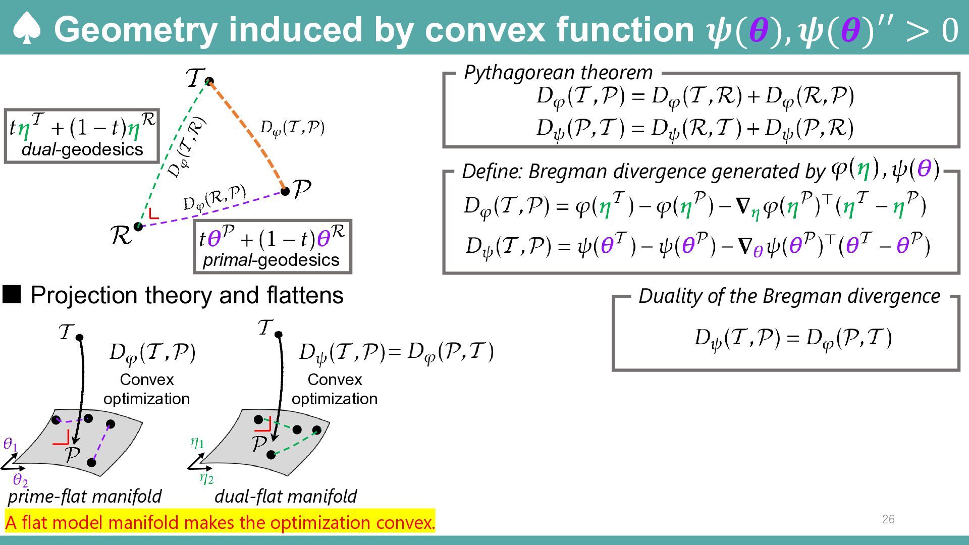
  25. Geometry induced by convex function 𝝍(𝜽), 𝝍(𝜽)′′ > 0 Pythagorean

    theorem dual-geodesics Define: Bregman divergence generated by primal-geodesics ▪ Projection theory and flattens Convex optimization Duality of the Bregman divergence Convex optimization dual-flat manifold prime-flat manifold A flat model manifold makes the optimization convex. 26
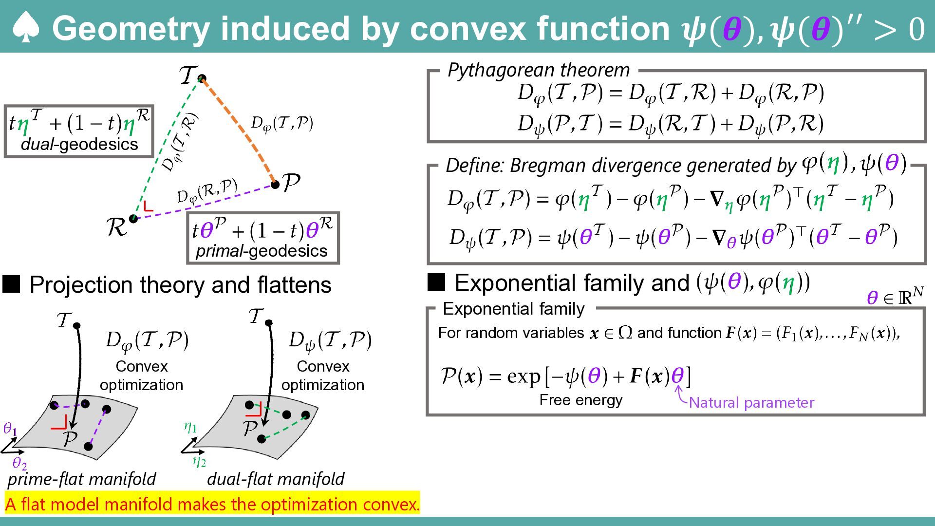
  26. Geometry induced by convex function 𝝍(𝜽), 𝝍(𝜽)′′ > 0 Pythagorean

    theorem dual-geodesics Define: Bregman divergence generated by primal-geodesics ▪ Projection theory and flattens ▪ Exponential family and Exponential family For random variables Convex optimization Convex optimization dual-flat manifold prime-flat manifold A flat model manifold makes the optimization convex. Free energy and function Natural parameter
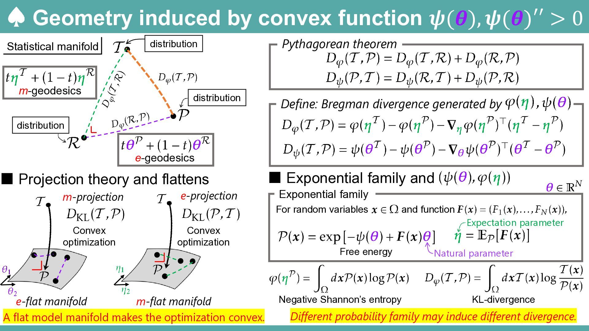
  27. Geometry induced by convex function 𝝍(𝜽), 𝝍(𝜽)′′ > 0 Statistical

    manifold m-geodesics distribution distribution Pythagorean theorem Define: Bregman divergence generated by distribution e-geodesics ▪ Projection theory and flattens m-projection e-projection ▪ Exponential family and Exponential family For random variables Convex optimization Convex optimization m-flat manifold e-flat manifold A flat model manifold makes the optimization convex. and function Expectation parameter Free energy Negative Shannon’s entropy Natural parameter KL-divergence Different probability family may induce different divergence.
  28. Non-negative normalized tensors as deformed exponential family -deformed-exponential family For

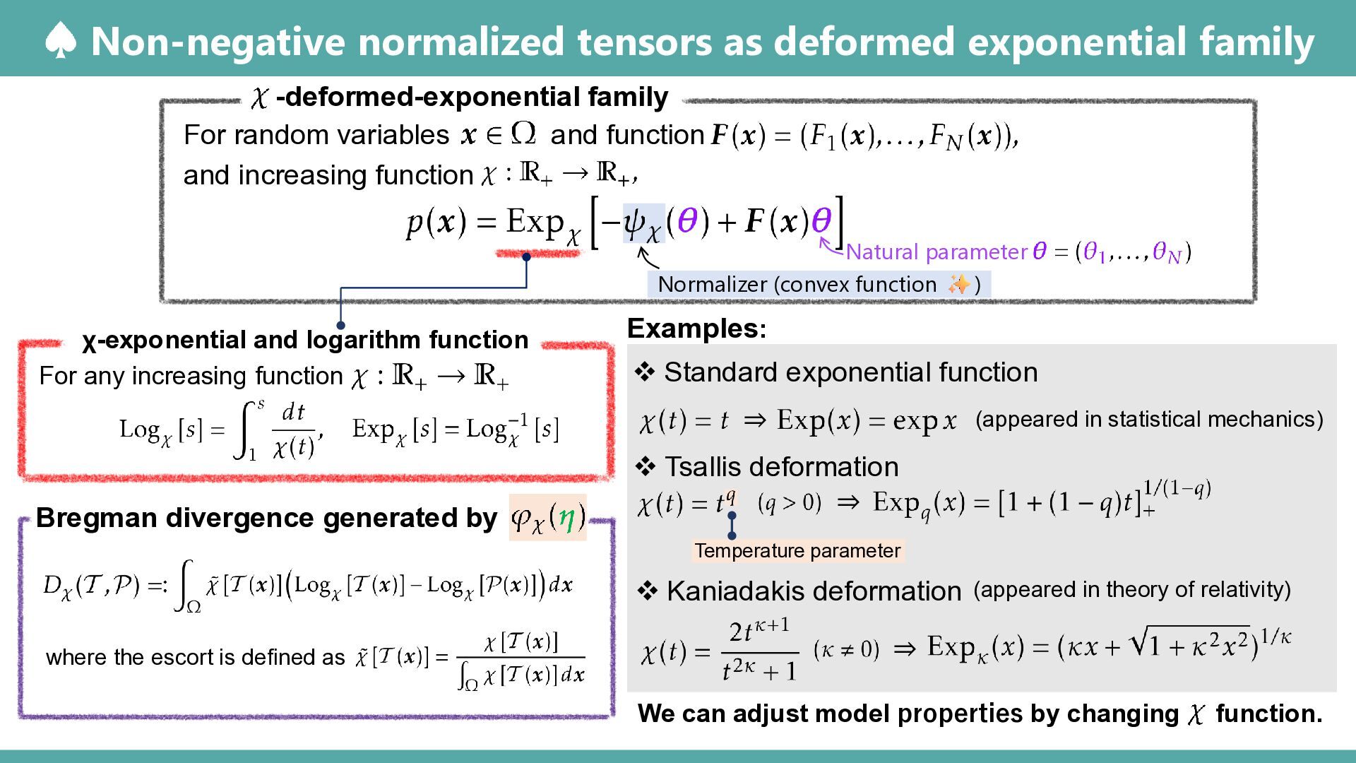
    random variables and function and increasing function Natural parameter Normalizer (convex function ) χ-exponential and logarithm function For any increasing function Examples: ❖ Standard exponential function ⇒ Bregman divergence generated by (appeared in statistical mechanics) ❖ Tsallis deformation ⇒ Temperature parameter ❖ Kaniadakis deformation (appeared in theory of relativity) where the escort is defined as ⇒ We can adjust model properties by changing function.
  29. Non-negative normalized tensors as deformed exponential family Natural parameter Normalizer

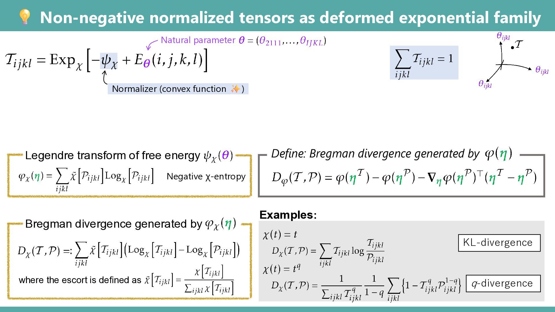
    (convex function ) Legendre transform of free energy Define: Bregman divergence generated by Negative χ-entropy Bregman divergence generated by Examples: KL-divergence where the escort is defined as q-divergence
  30. Deformed many-body approximation for non-negative tensors Energy function Natural parameter

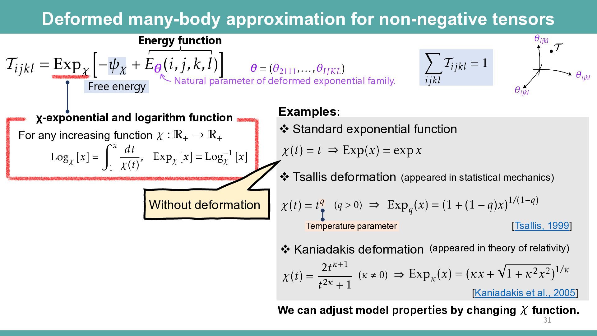
    of deformed exponential family. Free energy χ-exponential and logarithm function For any increasing function Examples: ❖ Standard exponential function ⇒ ❖ Tsallis deformation (appeared in statistical mechanics) Without deformation ⇒ Temperature parameter [Tsallis, 1999] ❖ Kaniadakis deformation (appeared in theory of relativity) ⇒ [Kaniadakis et al., 2005] We can adjust model properties by changing function. 31
  31. Deformed many-body approximation for non-negative tensors Natural parameter of deformed

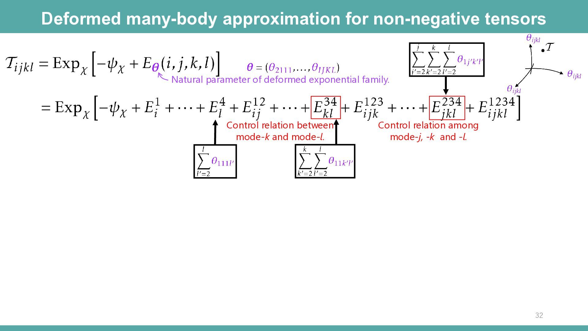
    exponential family. Control relation between mode-k and mode-l. Control relation among mode-j, -k and -l. 32
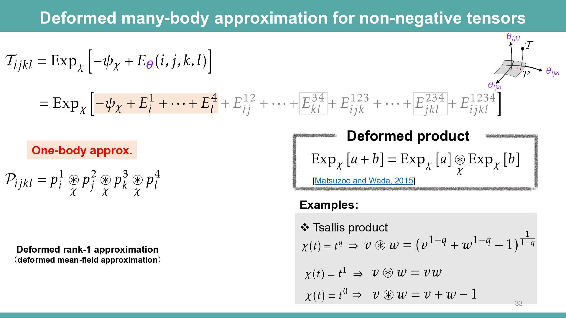
  32. Deformed many-body approximation for non-negative tensors One-body approx. Deformed product

    [Matsuzoe and Wada, 2015] Examples: ❖ Tsallis product Deformed rank-1 approximation ⇒ (deformed mean-field approximation) ⇒ ⇒ 33
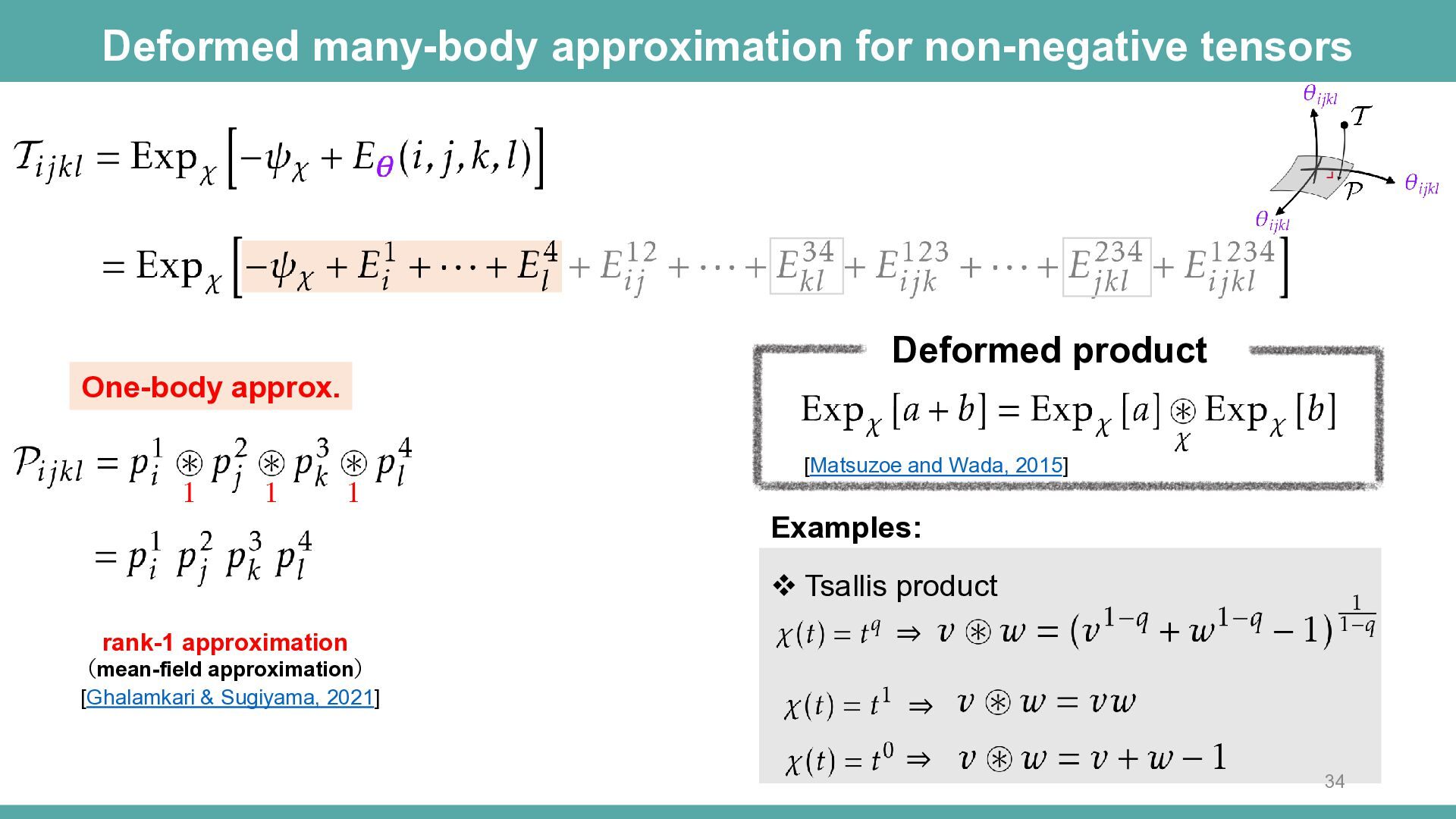
  33. Deformed many-body approximation for non-negative tensors One-body approx. Deformed product

    [Matsuzoe and Wada, 2015] Examples: ❖ Tsallis product rank-1 approximation (mean-field approximation) [Ghalamkari & Sugiyama, 2021] ⇒ ⇒ ⇒ 34
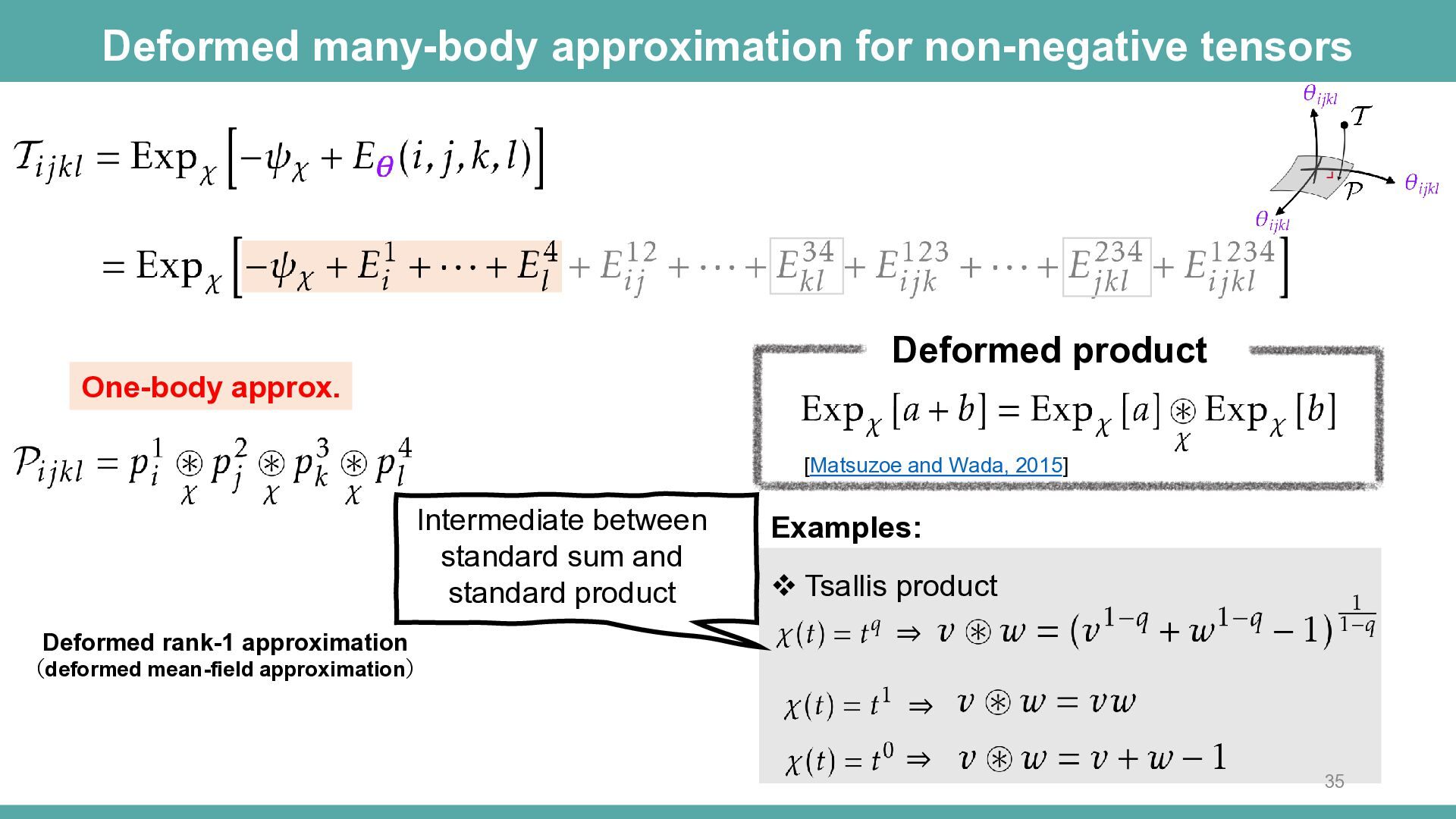
  34. Deformed many-body approximation for non-negative tensors Deformed product One-body approx.

    [Matsuzoe and Wada, 2015] Intermediate between standard sum and standard product Deformed rank-1 approximation Examples: ❖ Tsallis product ⇒ (deformed mean-field approximation) ⇒ ⇒ 35
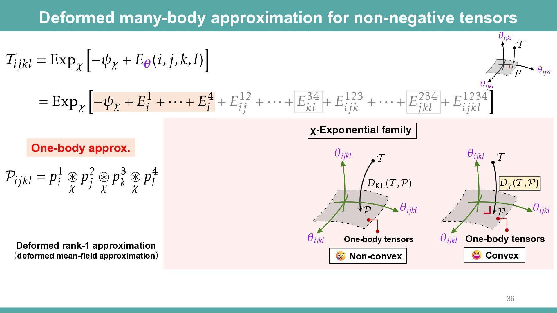
  35. Deformed many-body approximation for non-negative tensors χ-Exponential family One-body approx.

    Deformed rank-1 approximation (deformed mean-field approximation) One-body tensors One-body tensors Non-convex Convex 36
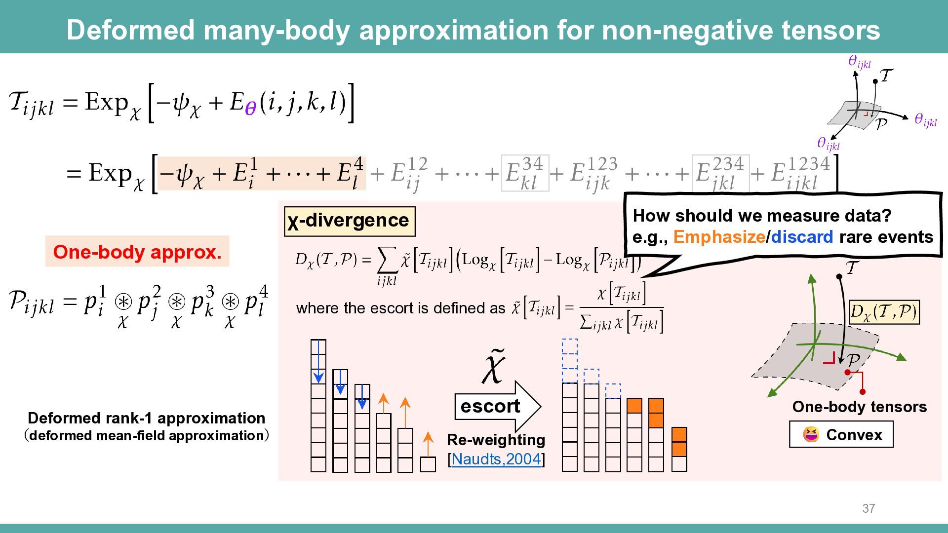
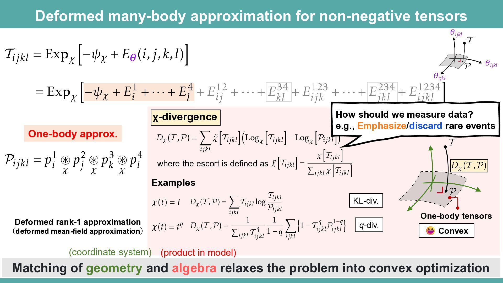
  36. Deformed many-body approximation for non-negative tensors How should we measure

    data? e.g., Emphasize/discard rare events χ-divergence One-body approx. where the escort is defined as Deformed rank-1 approximation (deformed mean-field approximation) escort One-body tensors Re-weighting [Naudts,2004] Convex 37
  37. Deformed many-body approximation for non-negative tensors χ-divergence One-body approx. How

    should we measure data? e.g., Emphasize/discard rare events where the escort is defined as Examples KL-div. Deformed rank-1 approximation (deformed mean-field approximation) q-div. One-body tensors Convex (coordinate system) (product in model) Matching of geometry and algebra relaxes the problem into convex optimization
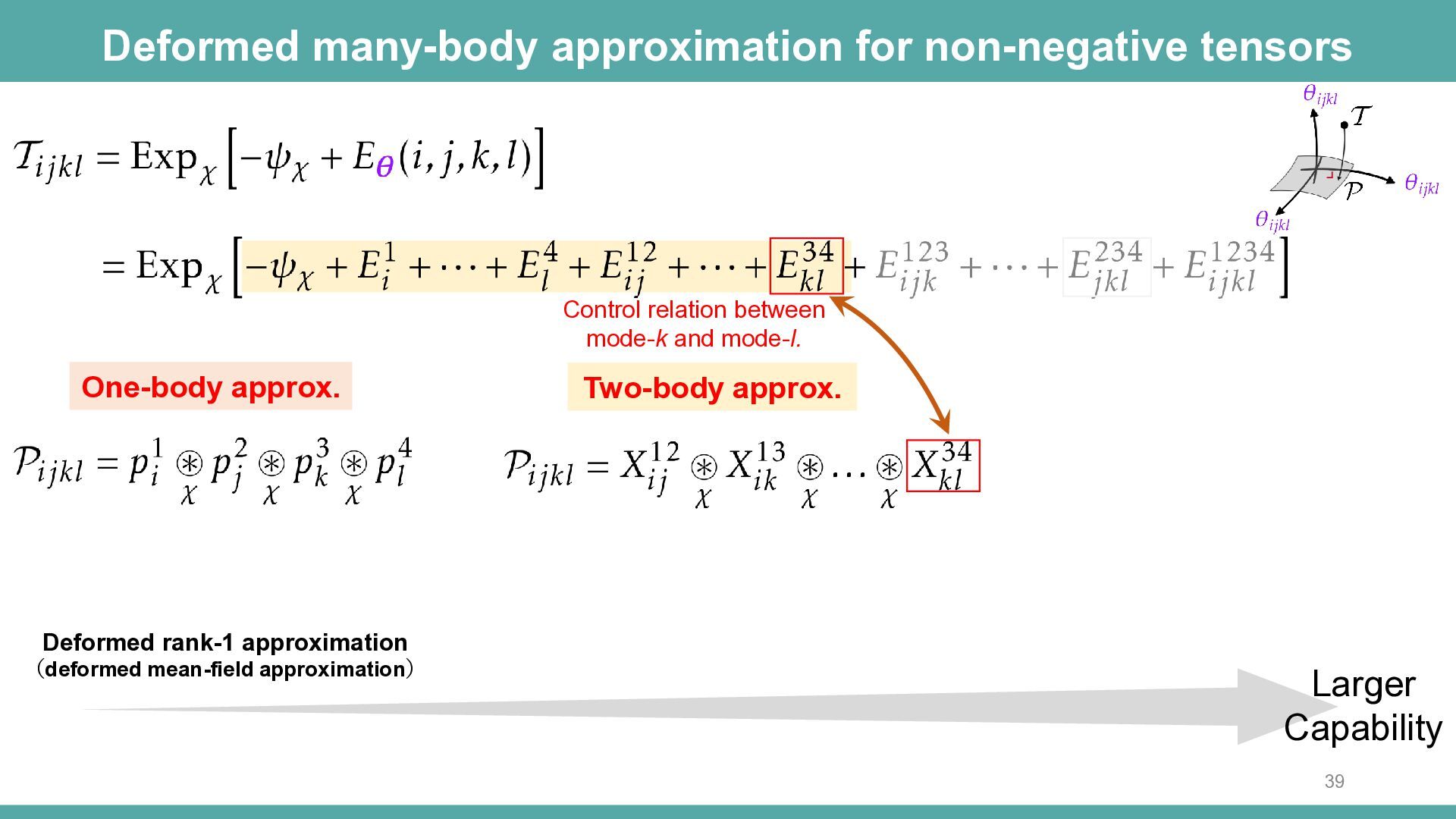
  38. Deformed many-body approximation for non-negative tensors Control relation between mode-k

    and mode-l. One-body approx. Two-body approx. Deformed rank-1 approximation (deformed mean-field approximation) Larger Capability 39
  39. Deformed many-body approximation for non-negative tensors [Ghalamkari et. al, 2026]

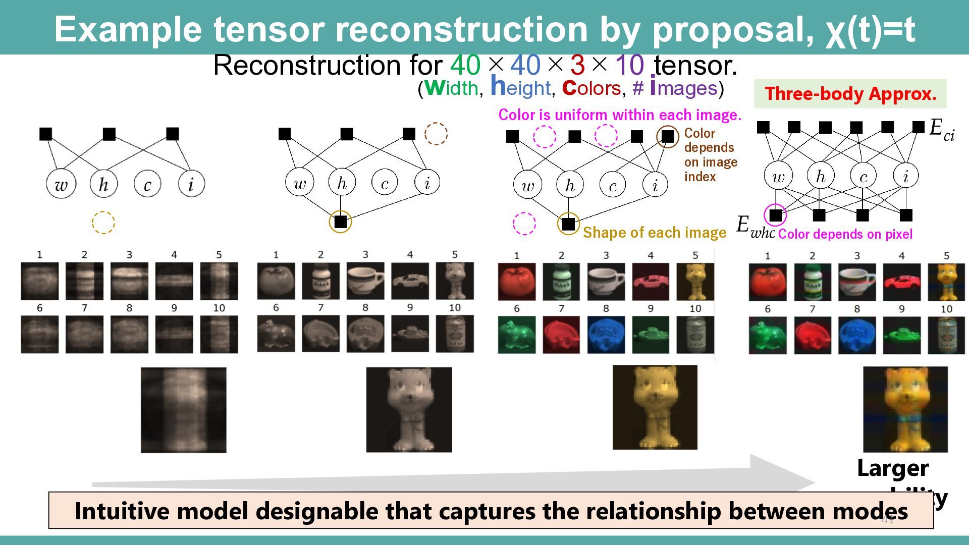
    Control relation between mode-k and mode-l. One-body approx. Control relation among mode-j, -k and -l. Three-body approx. Two-body approx. Two-body Interaction Three-body Interaction Deformed rank-1 approximation (deformed mean-field approximation) Intuitive modeling focusing on interactions between modes The global optimal solution minimizing from Larger Capability can be obtained by a convex optimization. 40
  40. Example tensor reconstruction by proposal, χ(t)=t Reconstruction for 40×40×3×10 tensor.

    (width, height, colors, # images) Three-body Approx. Color is uniform within each image. Color depends on image index Shape of each image Color depends on pixel Larger capability Intuitive model designable that captures the relationship between modes 41
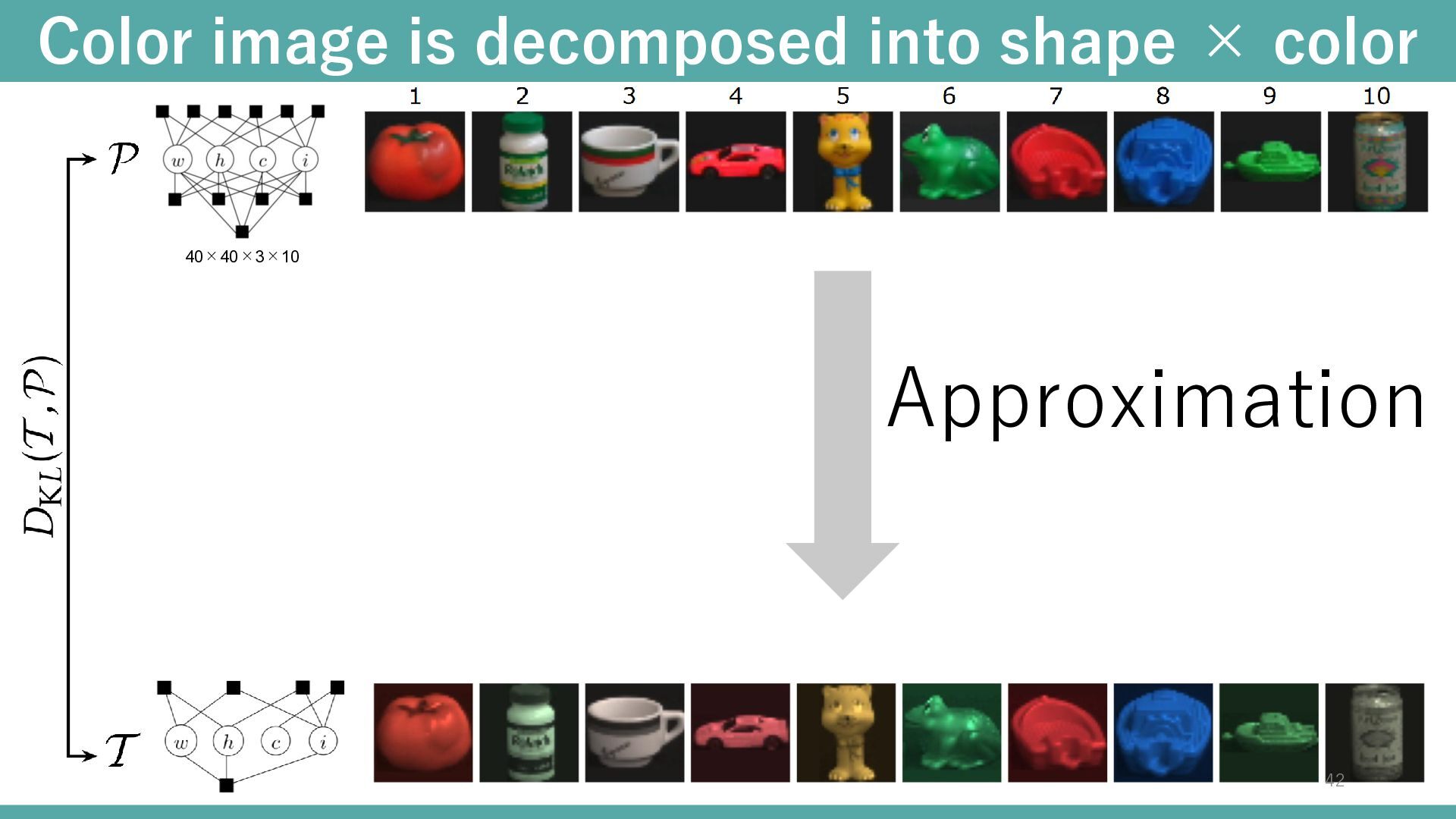
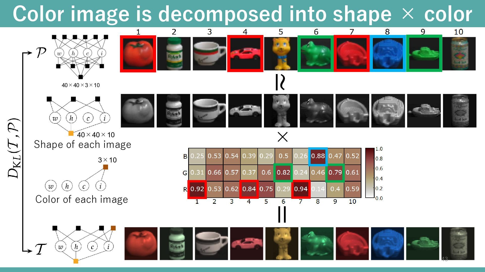
  41. Color image is decomposed into shape × color 40×40×10 Shape

    of each image ≃ 40×40×3×10 × 3×10 Color of each image = 43
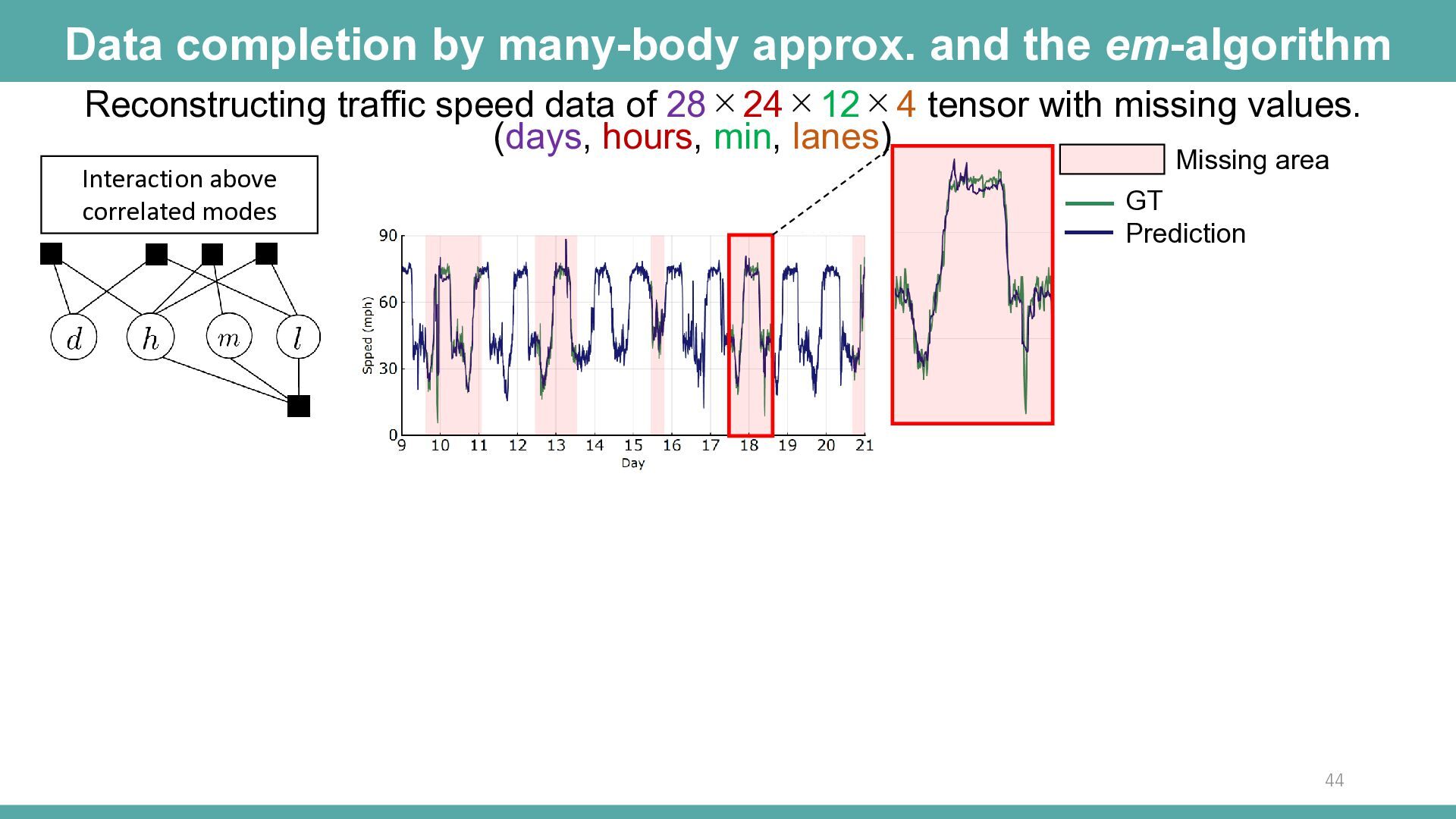
  42. Data completion by many-body approx. and the em-algorithm Reconstructing traffic

    speed data of 28×24×12×4 tensor with missing values. (days, hours, min, lanes) Interaction above correlated modes Missing area GT Prediction 44
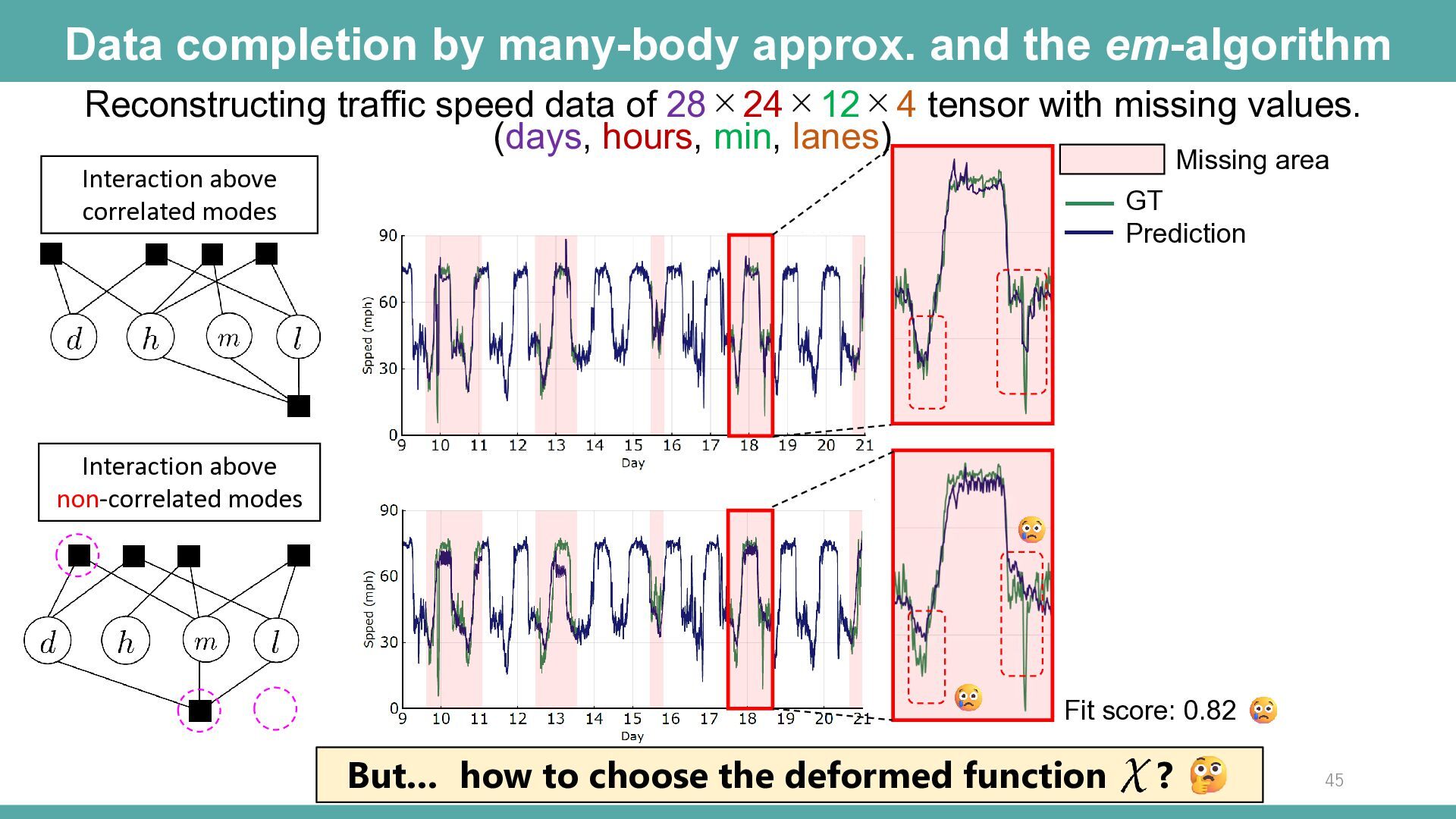
  43. Data completion by many-body approx. and the em-algorithm Reconstructing traffic

    speed data of 28×24×12×4 tensor with missing values. (days, hours, min, lanes) Missing area Interaction above correlated modes GT Prediction Interaction above non-correlated modes Fit score: 0.82 But… how to choose the deformed function ? 45
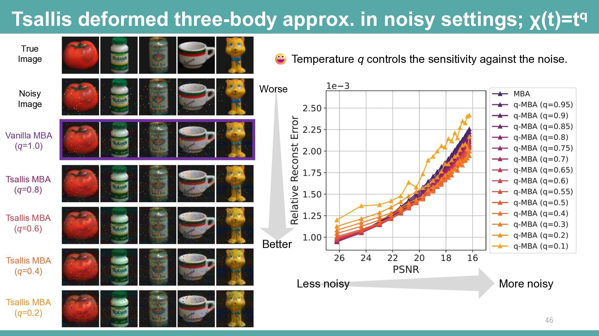
  44. Tsallis deformed three-body approx. in noisy settings; χ(t)=tq True Image

    Noisy Image Temperature q controls the sensitivity against the noise. Worse Vanilla MBA (q=1.0) Tsallis MBA (q=0.8) Tsallis MBA (q=0.6) Better Tsallis MBA (q=0.4) Less noisy Tsallis MBA (q=0.2) More noisy 46
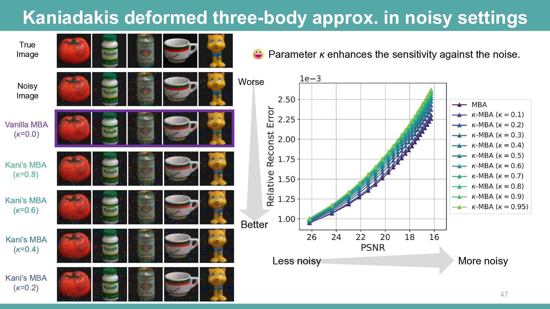
  45. Kaniadakis deformed three-body approx. in noisy settings True Image Noisy

    Image Parameter κ enhances the sensitivity against the noise. Worse Vanilla MBA (κ=0.0) Kani’s MBA (κ=0.8) Kani’s MBA (κ=0.6) Better Kani’s MBA (κ=0.4) Less noisy Kani’s MBA (κ=0.2) More noisy 47
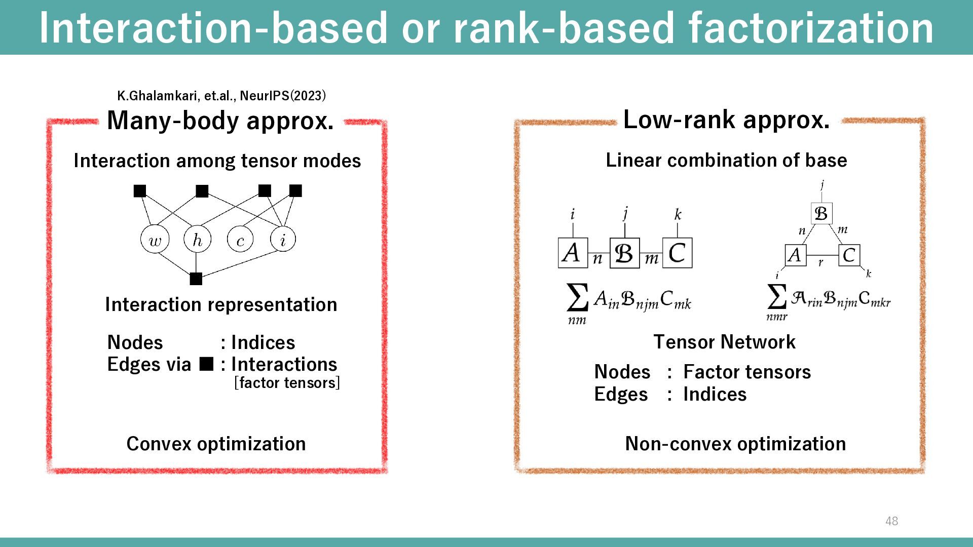
  46. Interaction-based or rank-based factorization K.Ghalamkari, et.al., NeurIPS(2023) Many-body approx. Low-rank

    approx. Interaction among tensor modes Linear combination of base Interaction representation Nodes : Indices Edges via ▪ : Interactions [factor tensors] Convex optimization Tensor Network Nodes : Factor tensors Edges : Indices Non-convex optimization 48
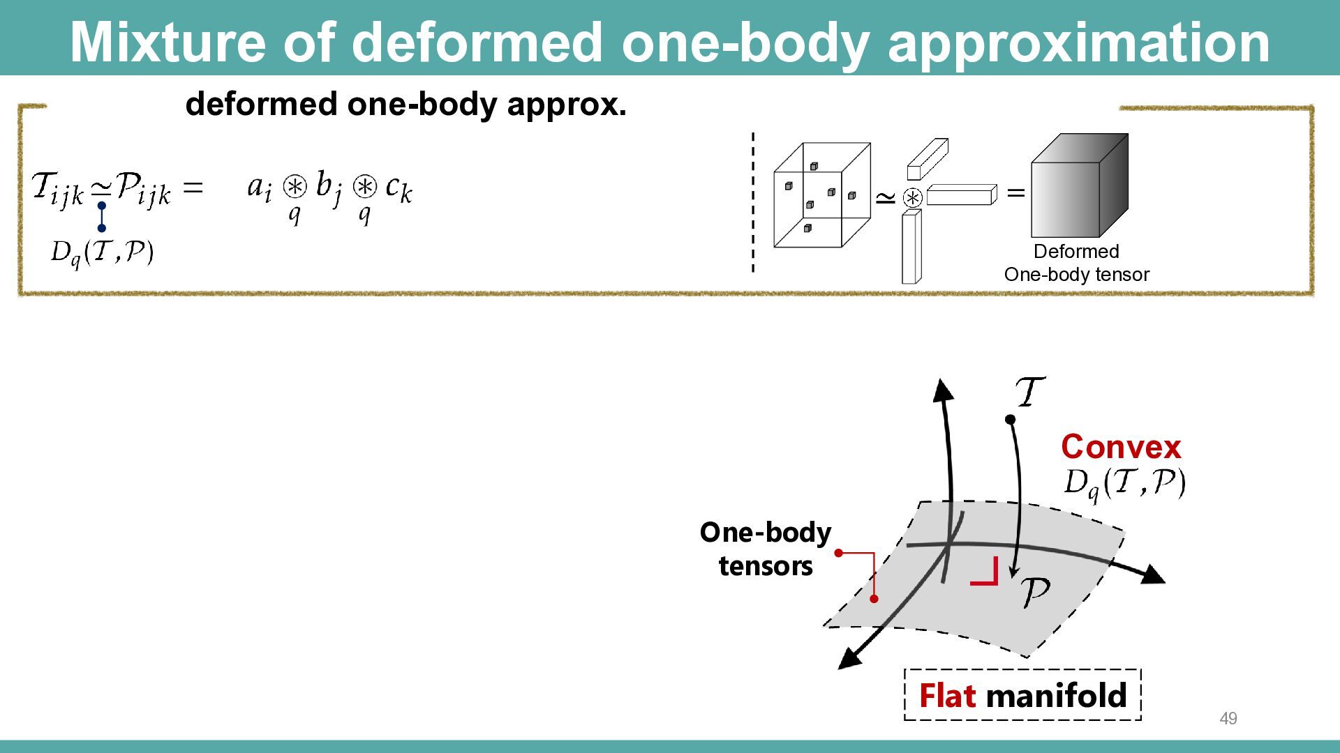
  47. Mixture of deformed one-body approximation deformed one-body approx. = Deformed

    One-body tensor Convex One-body tensors Flat manifold 49
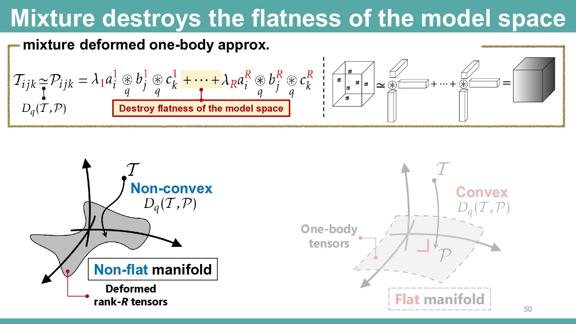
  48. Mixture destroys the flatness of the model space mixture deformed

    one-body approx. +⋯+ = Destroy flatness of the model space Non-convex Convex One-body tensors Non-flat manifold Deformed rank-R tensors Flat manifold 50
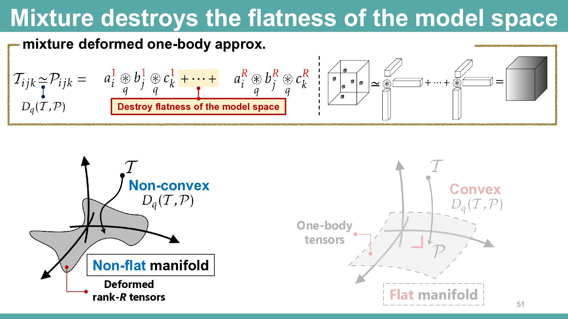
  49. Mixture destroys the flatness of the model space mixture deformed

    one-body approx. +⋯+ = Destroy flatness of the model space Non-convex Convex One-body tensors Non-flat manifold Deformed rank-R tensors Flat manifold 51
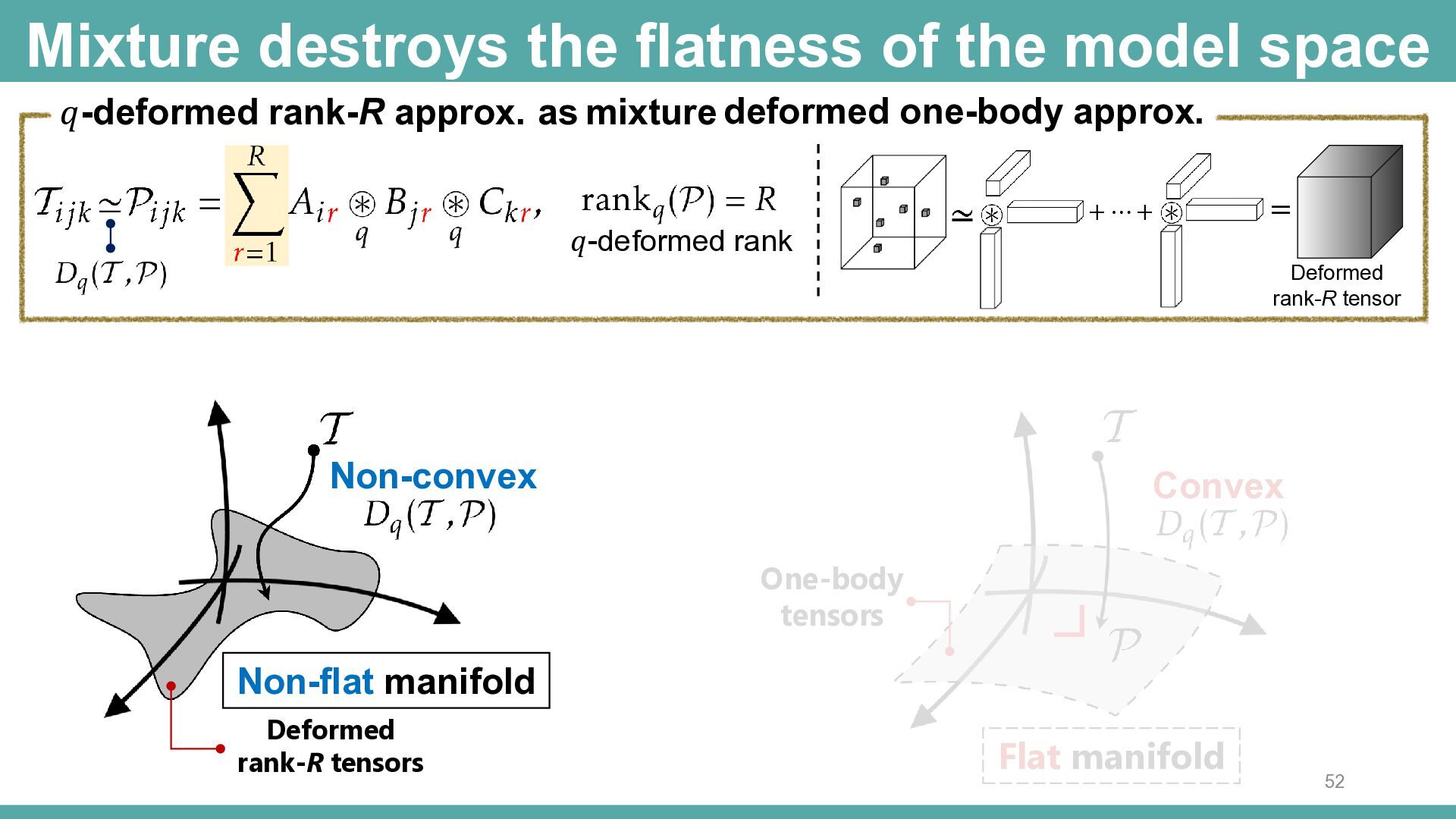
  50. Mixture destroys the flatness of the model space 𝑞-deformed rank-R

    approx. as mixture deformed one-body approx. 𝑞-deformed rank +⋯+ = Deformed rank-R tensor Non-convex Convex One-body tensors Non-flat manifold Deformed rank-R tensors Flat manifold 52
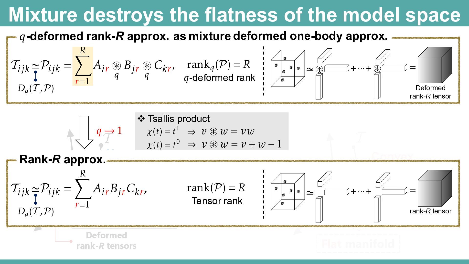
  51. Mixture destroys the flatness of the model space 𝑞-deformed rank-R

    approx. as mixture deformed one-body approx. 𝑞-deformed rank +⋯+ = Deformed rank-R tensor ❖ Tsallis product ⇒ ⇒ Rank-R approx.Non-convex Convex One-body Tensor rank tensors +⋯+ rank-R tensor Non-flat manifold Deformed rank-R tensors = Flat manifold
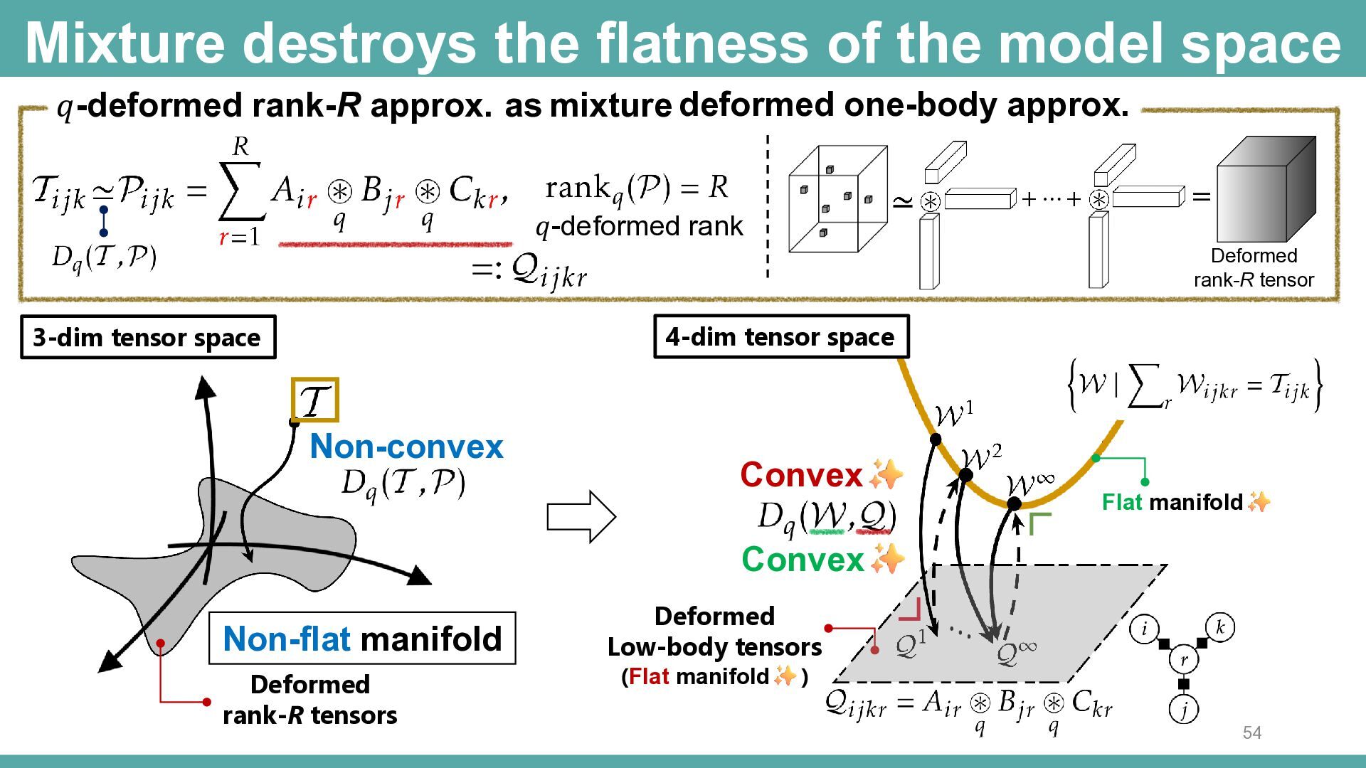
  52. Mixture destroys the flatness of the model space 𝑞-deformed rank-R

    approx. as mixture deformed one-body approx. +⋯+ 𝑞-deformed rank = Deformed rank-R tensor 4-dim tensor space 3-dim tensor space Non-convex Convex Flat manifold Convex Non-flat manifold Deformed rank-R tensors Deformed Low-body tensors (Flat manifold ) 54
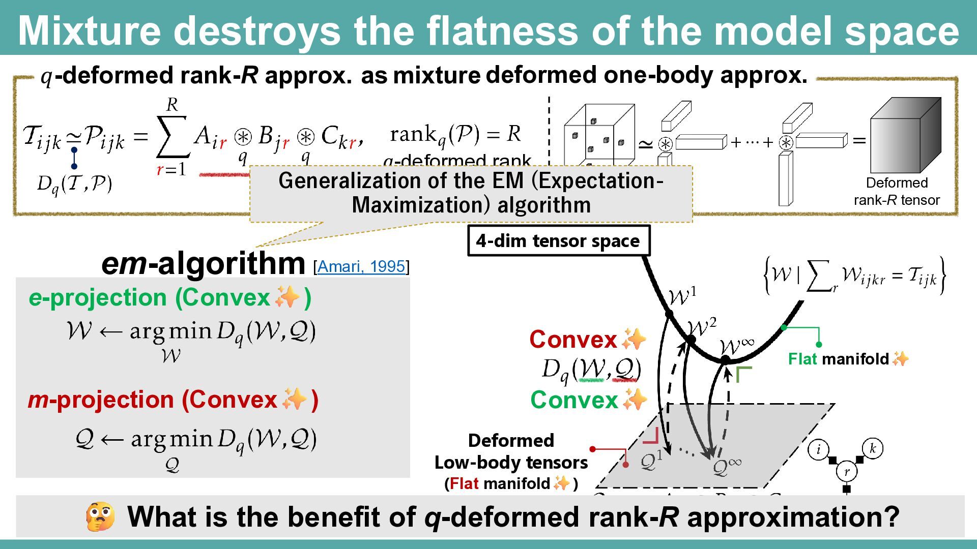
  53. Mixture destroys the flatness of the model space 𝑞-deformed rank-R

    approx. as mixture deformed one-body approx. 𝑞-deformed rank Generalization of the EM (ExpectationMaximization) algorithm em-algorithm [Amari, 1995] e-projection (Convex = Deformed rank-R tensor 4-dim tensor space ) Convex m-projection (Convex +⋯+ ) Flat manifold Convex Deformed Low-body tensors (Flat manifold ) What is the benefit of q-deformed rank-R approximation?55
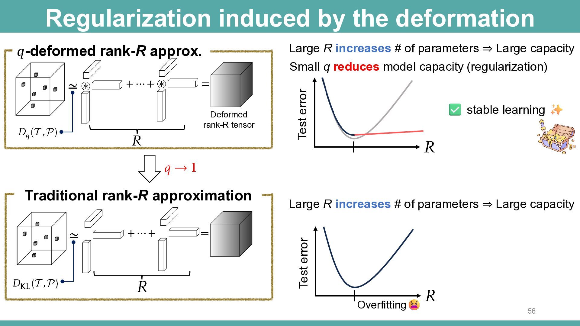
  54. Regularization induced by the deformation Large R increases # of

    parameters ⇒ Large capacity 𝑞-deformed rank-R approx. = Deformed rank-R tensor Traditional rank-R approximation +⋯+ = stable learning Large R increases # of parameters ⇒ Large capacity Test error +⋯+ Test error Small q reduces model capacity (regularization) Overfitting 56
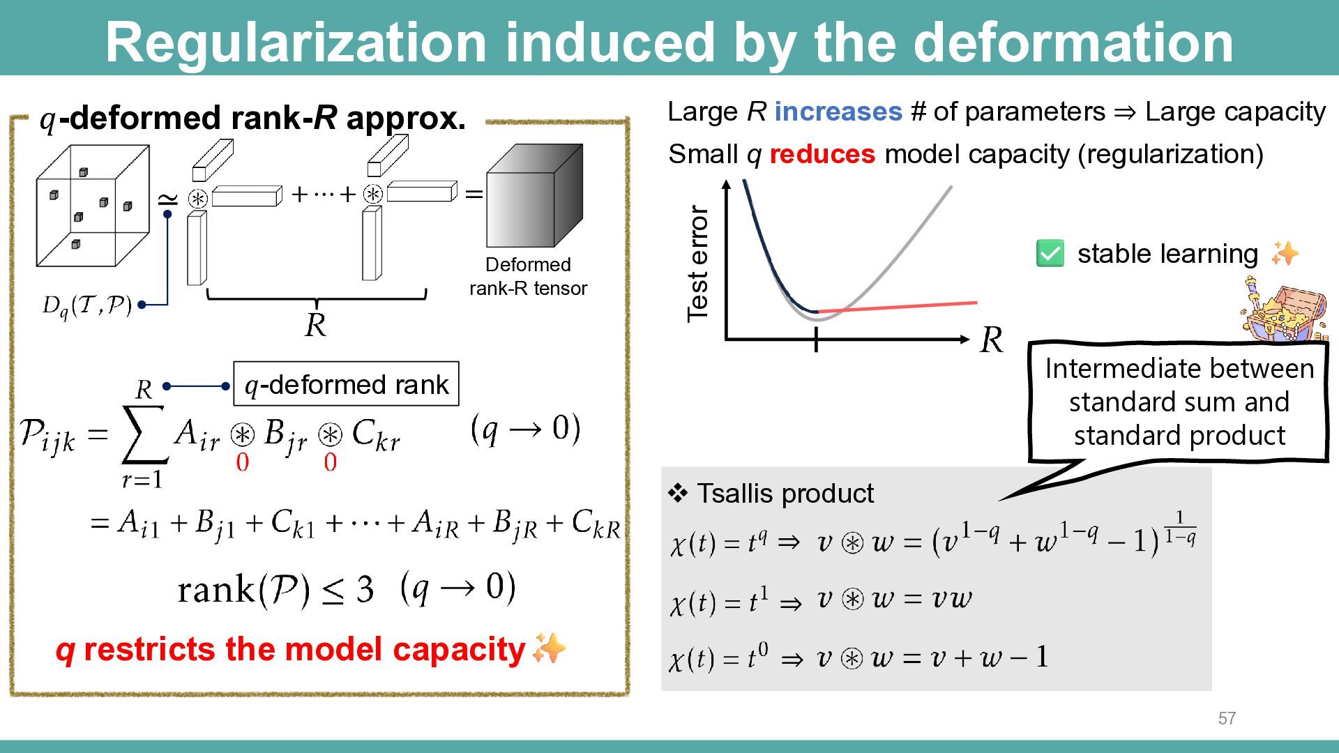
  55. Regularization induced by the deformation Large R increases # of

    parameters ⇒ Large capacity 𝑞-deformed rank-R approx. +⋯+ = Deformed rank-R tensor Test error Small q reduces model capacity (regularization) stable learning Intermediate between standard sum and standard product 𝑞-deformed rank ❖ Tsallis product ⇒ ⇒ q restricts the model capacity ⇒ 57
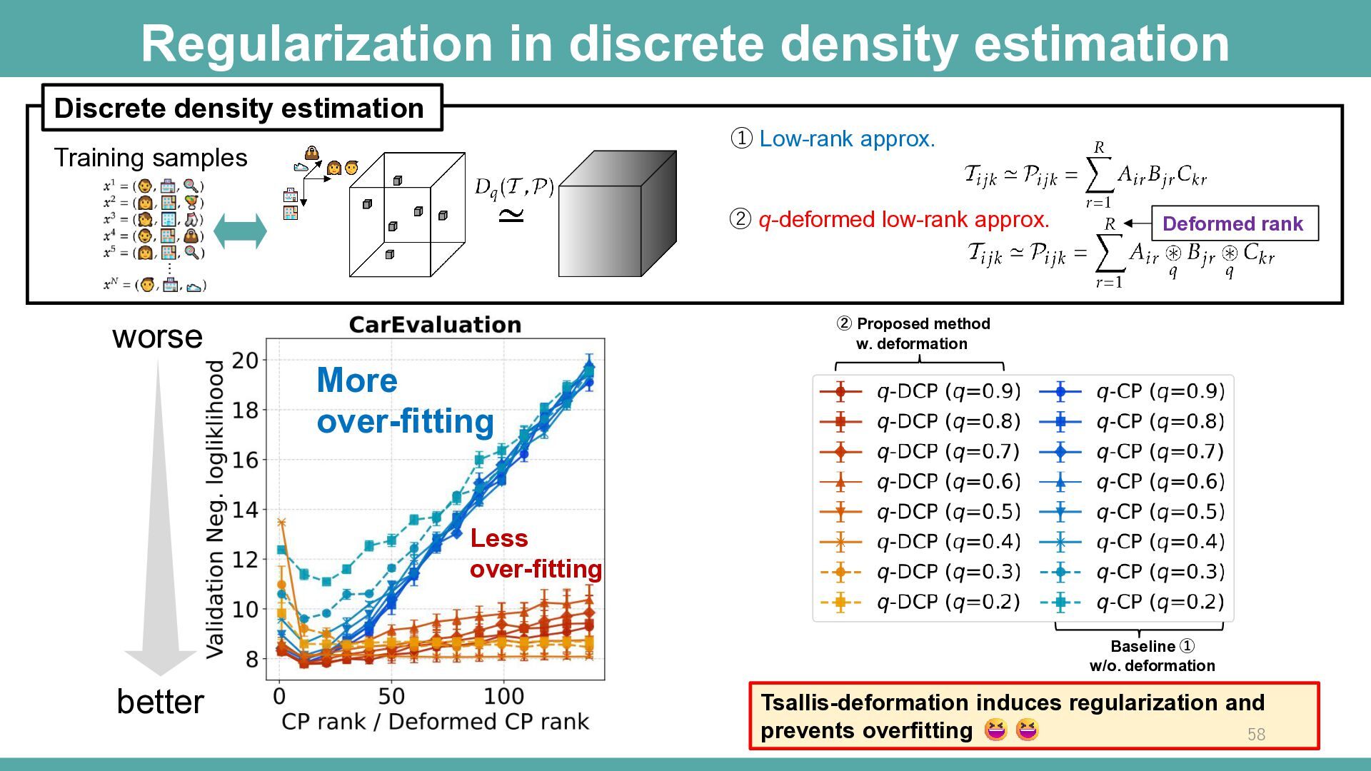
  56. Regularization in discrete density estimation Discrete density estimation ① Low-rank

    approx. Training samples ② q-deformed low-rank approx. Deformed rank ② Proposed method w. deformation worse More over-fitting Less over-fitting Baseline ① w/o. deformation better Tsallis-deformation induces regularization and prevents overfitting 58
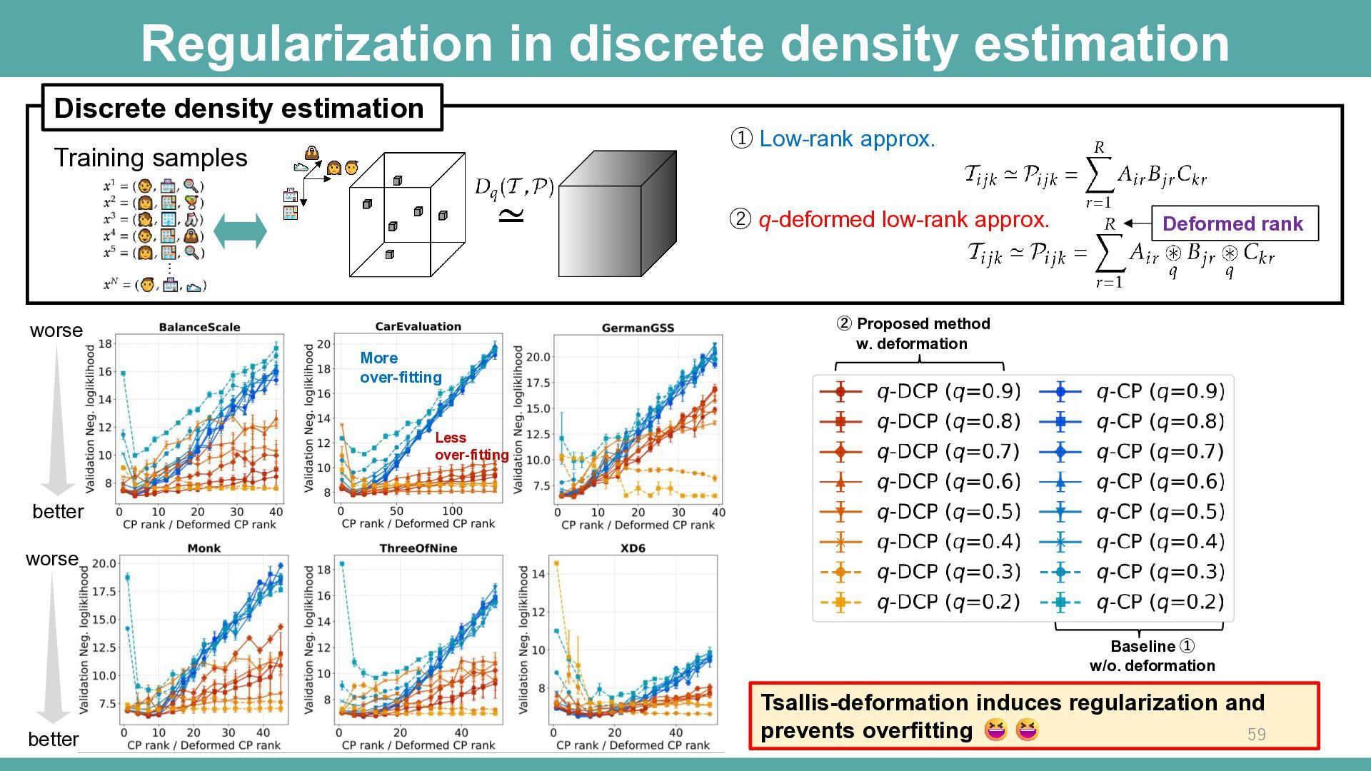
  57. Regularization in discrete density estimation Discrete density estimation ① Low-rank

    approx. Training samples ② q-deformed low-rank approx. worse More over-fitting Deformed rank ② Proposed method w. deformation Less over-fitting better worse Baseline ① w/o. deformation better Tsallis-deformation induces regularization and prevents overfitting 59
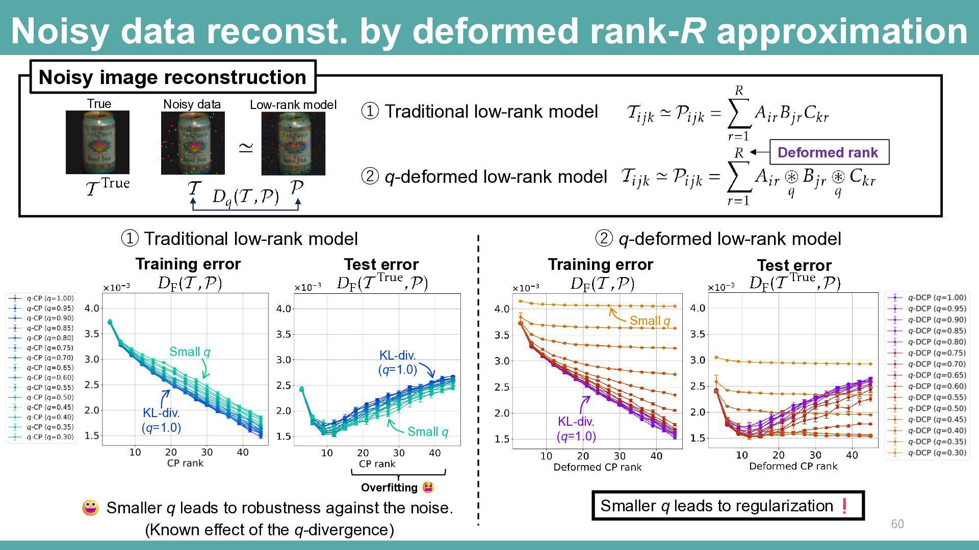
  58. Noisy data reconst. by deformed rank-R approximation Noisy image reconstruction

    True Noisy data Low-rank model ① Traditional low-rank model Deformed rank ② q-deformed low-rank model ② q-deformed low-rank model ① Traditional low-rank model Training error Test error Training error Test error Small q Small q KL-div. (q=1.0) KL-div. (q=1.0) Small q KL-div. (q=1.0) Overfitting Smaller q leads to robustness against the noise. (Known effect of the q-divergence) Smaller q leads to regularization 60
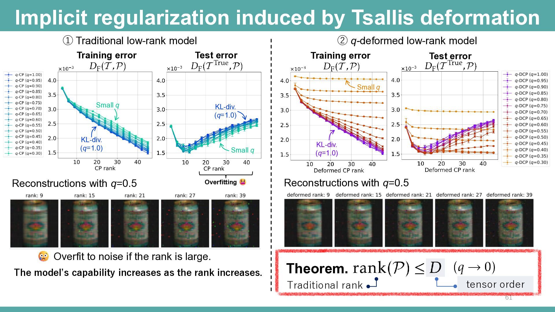
  59. Implicit regularization induced by Tsallis deformation ① Traditional low-rank model

    Training error ② q-deformed low-rank model Test error Training error Test error Small q Small q KL-div. (q=1.0) KL-div. (q=1.0) Reconstructions with q=0.5 Small q Overfitting Overfit to noise if the rank is large. The model’s capability increases as the rank increases. KL-div. (q=1.0) Reconstructions with q=0.5 No noise even with larger ranks Theorem. For small 𝑞, the model capacity remains limited despite a large deformed rank. tensor order Traditional rank 61
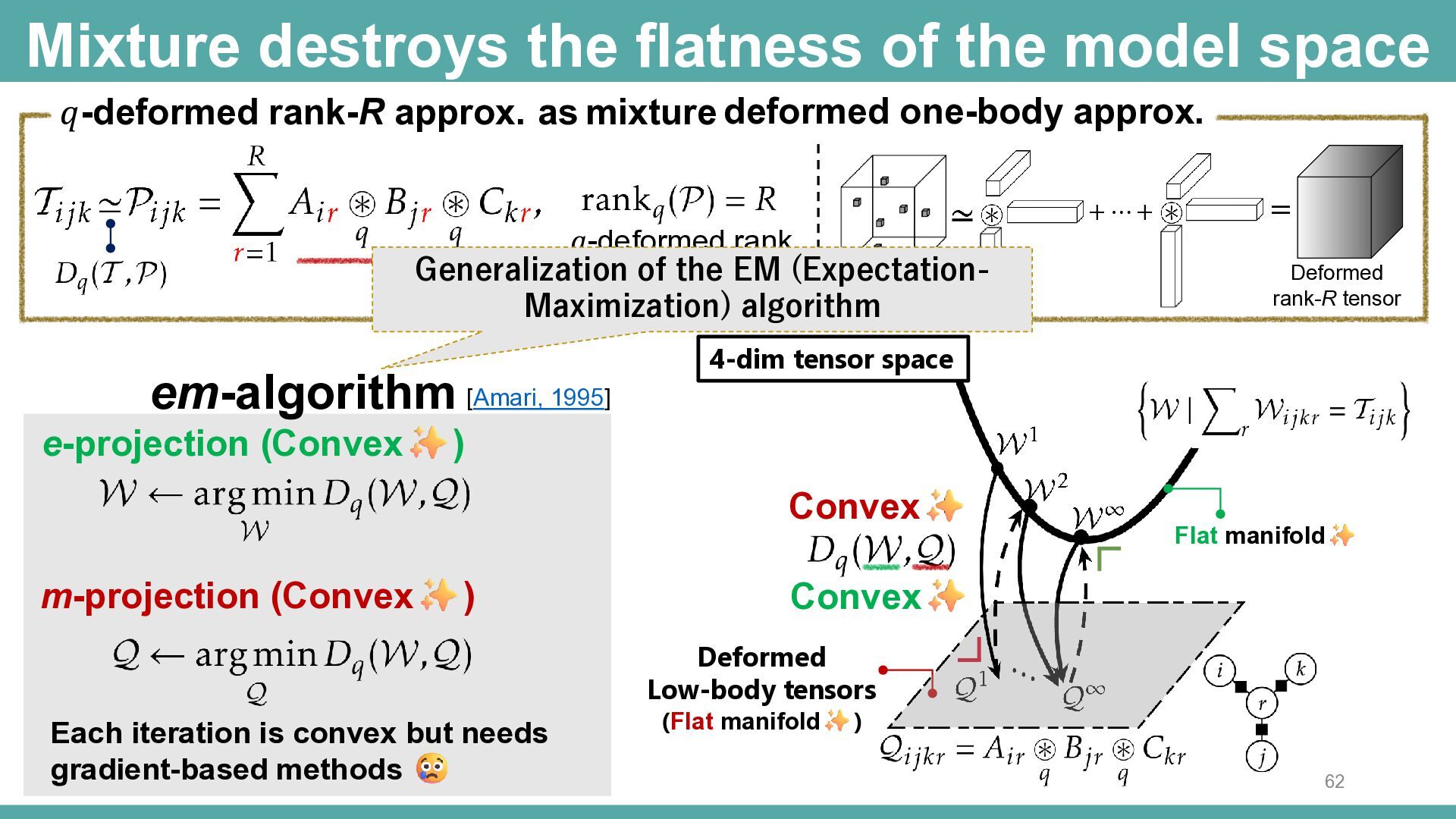
  60. Mixture destroys the flatness of the model space 𝑞-deformed rank-R

    approx. as mixture deformed one-body approx. 𝑞-deformed rank Generalization of the EM (ExpectationMaximization) algorithm em-algorithm [Amari, 1995] e-projection (Convex = Deformed rank-R tensor 4-dim tensor space ) Convex m-projection (Convex +⋯+ ) Flat manifold Convex Deformed Low-body tensors Each iteration is convex but needs gradient-based methods (Flat manifold ) 62
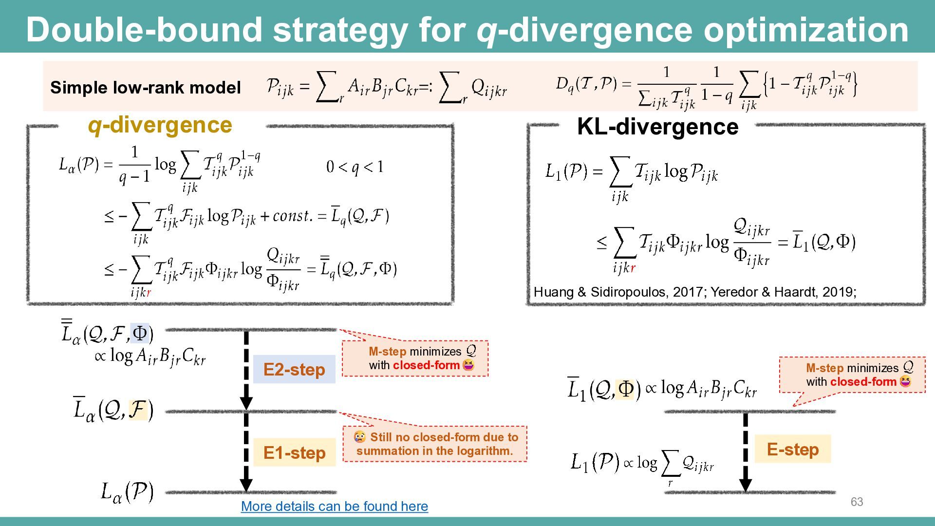
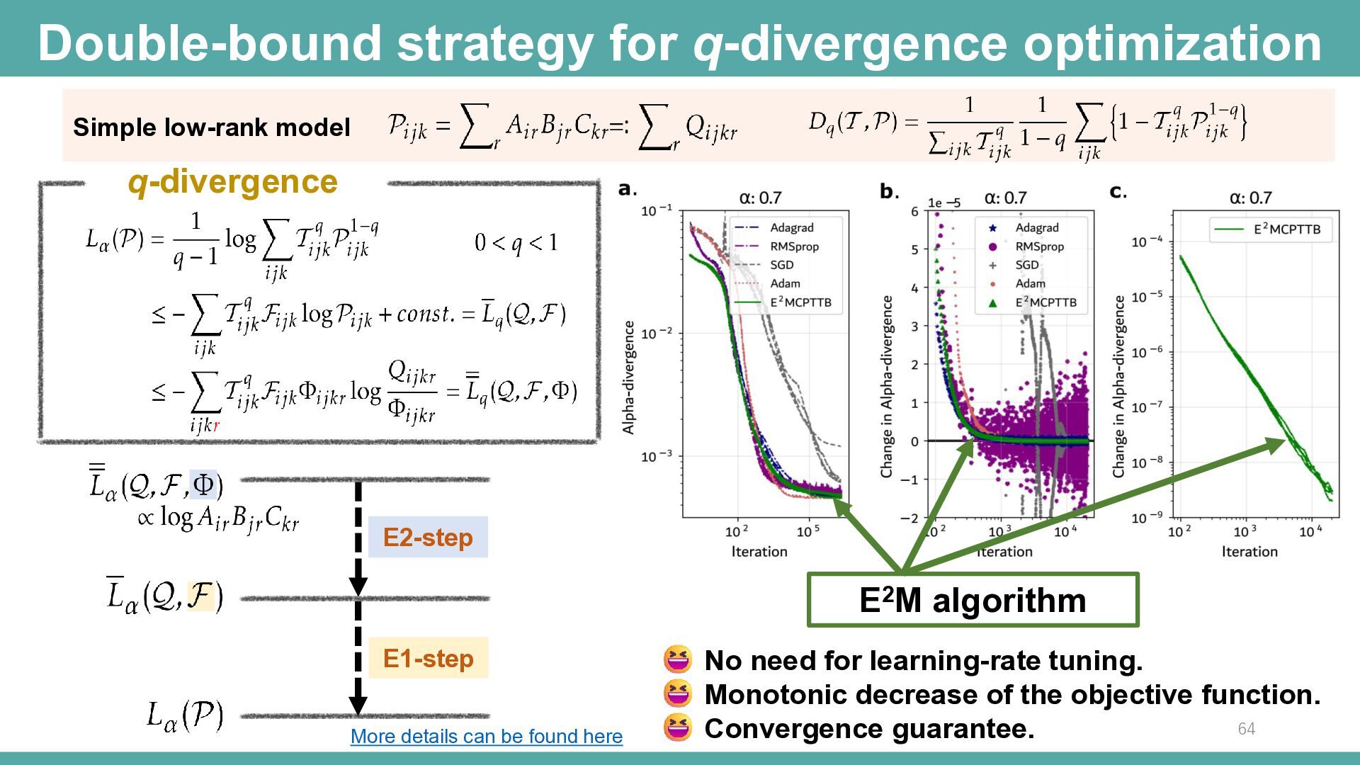
  61. Double-bound strategy for q-divergence optimization Simple low-rank model q-divergence KL-divergence

    Huang & Sidiropoulos, 2017; Yeredor & Haardt, 2019; E2-step E1-step M-step minimizes with closed-form Still no closed-form due to summation in the logarithm. More details can be found here M-step minimizes with closed-form E-step 63
  62. Double-bound strategy for q-divergence optimization Simple low-rank model q-divergence E2-step

    E2M algorithm E1-step More details can be found here No need for learning-rate tuning. Monotonic decrease of the objective function. 64 Convergence guarantee.
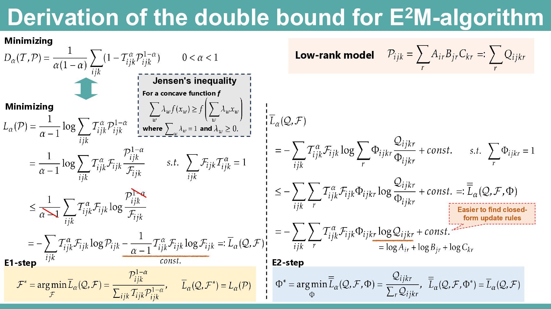
  63. Derivation of the double bound for E2M-algorithm Minimizing Low-rank model

    Jensen's inequality For a concave function f Minimizing where and Easier to find closedform update rules E1-step E2-step
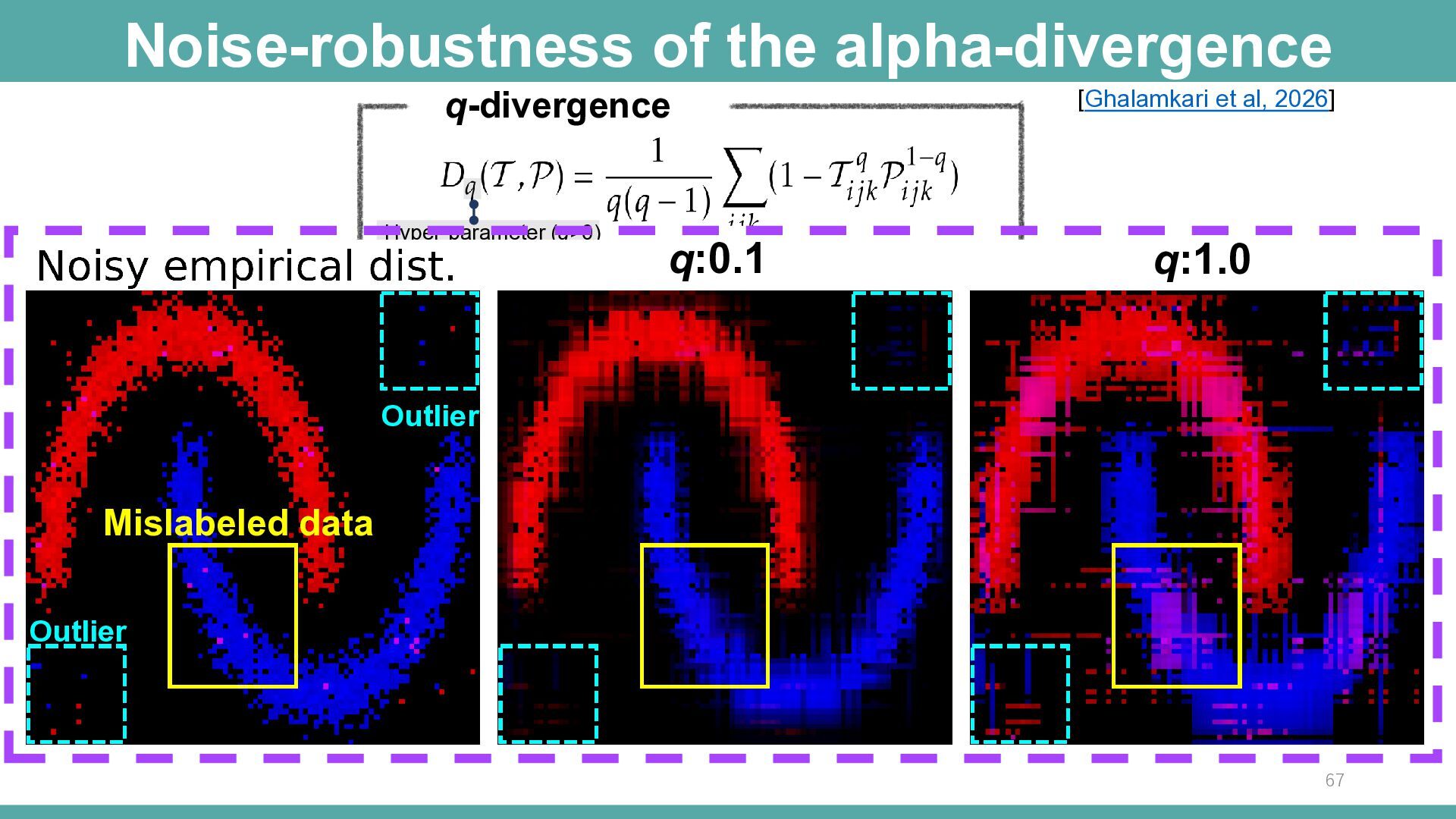
  64. Noise-robustness of the alpha-divergence q-divergence [Ghalamkari et al, 2026] Hyper-parameter

    (q>0) Reconstructed rank 30 CP tensor P with varying q. Observed T q:0.1 q:0.3 q:0.5 q:0.7 q:1.0 True distribution class A T with 50 noise class B 90 × 90 × 2 tensor 66
  65. Noise-robustness of the alpha-divergence q-divergence Hyper-parameter (q>0) [Ghalamkari et al,

    2026] q:0.1 q:1.0 Reconstructed rank 30 CP tensor P with varying q. Observed T True distribution class A q:0.1 q:0.3 q:0.5 q:0.7 q:1.0 Outlier Mislabeled data T with 50 noise class B 90 × 90 × 2 tensor Outlier 67
  66. Noise-robustness of the alpha-divergence q-divergence [Ghalamkari et al, 2026] Hyper-parameter

    (q>0) Reconstructed rank 30 CP tensor P with varying q. Observed T q:0.1 q:0.3 q:0.5 q:0.7 q:1.0 True distribution class A T with 50 noise class B 90 × 90 × 2 tensor Noise robust Noise sensitive 68 We can adjust the sensitivity to outliers and noise by the hyperparameter q.
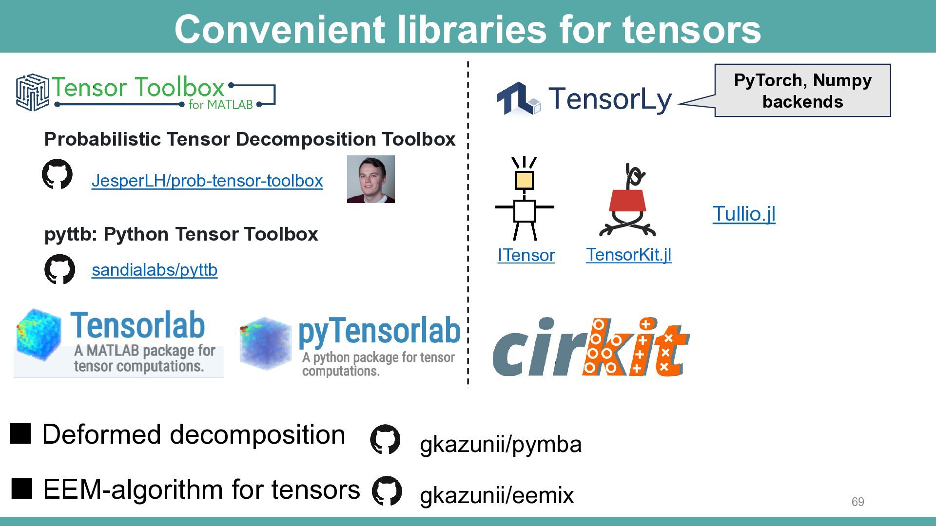
  67. Convenient libraries for tensors PyTorch, Numpy backends ロゴ 自動的に生成さ れた説明

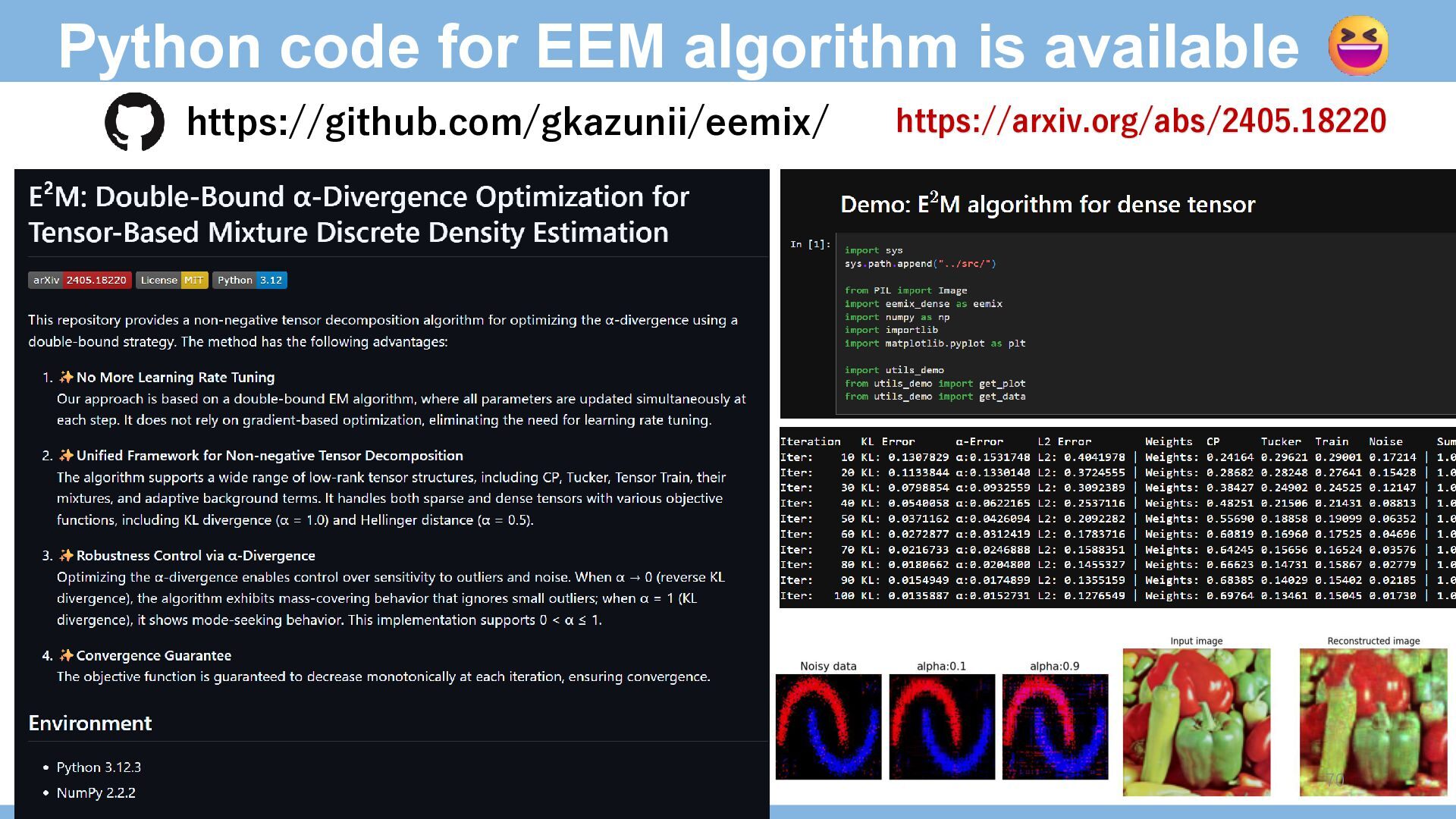
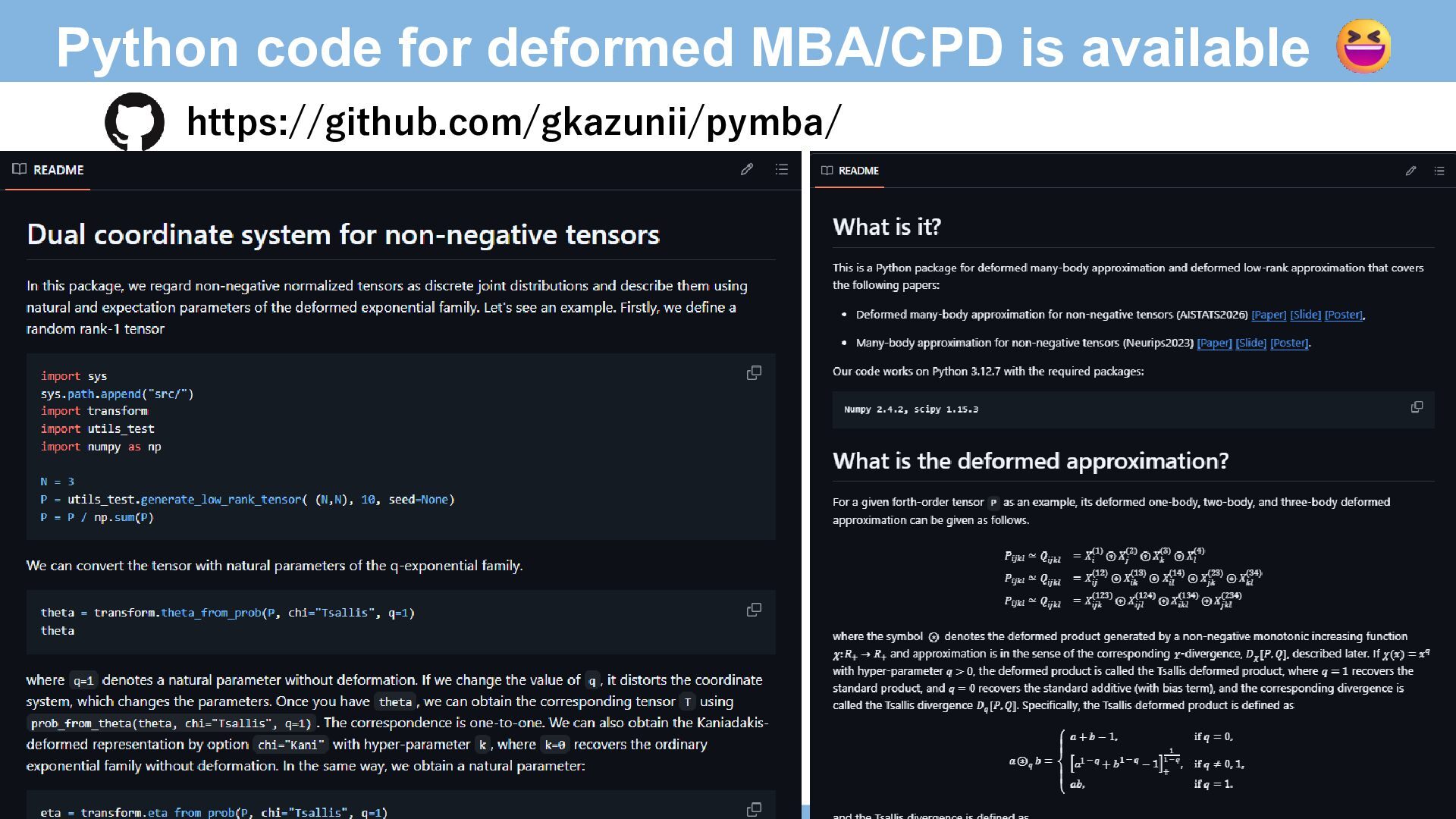
    Probabilistic Tensor Decomposition Toolbox 箱ひげ図が含まれている画像 自動的に生成さ れた説明 JesperLH/prob-tensor-toolbox Tullio.jl pyttb: Python Tensor Toolbox sandialabs/pyttb ITensor ▪ Deformed decomposition gkazunii/pymba ▪ EEM-algorithm for tensors gkazunii/eemix TensorKit.jl 69
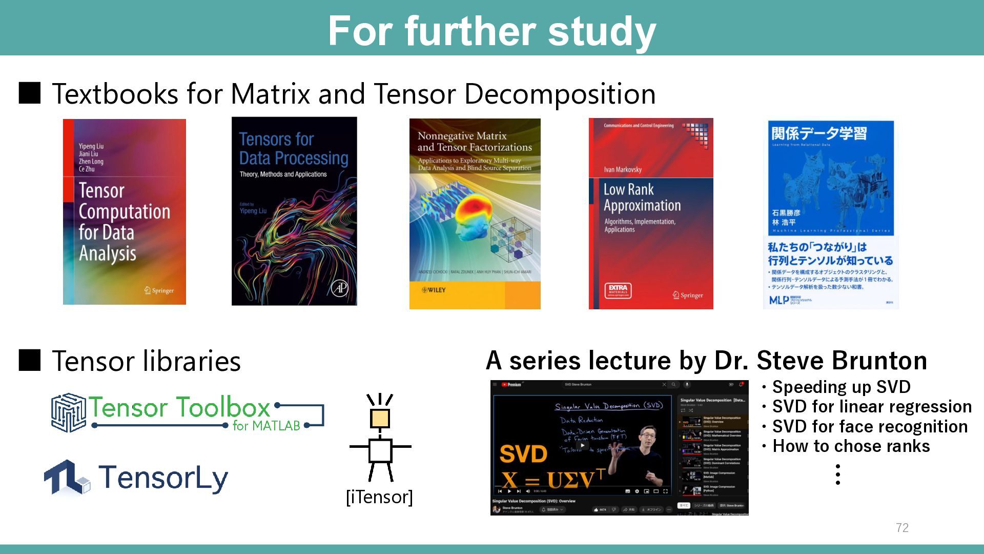
  68. For further study ▪ Textbooks for Matrix and Tensor Decomposition

    テキストが含まれている画像 自動的に生成された説明 カ レンダー 中程度の精度で自動的に生成さ れた説明 グラフィ カルユーザーインターフェ イス 自動的に生成された説明 ▪ Tensor libraries ,記 時 メ ボ ー 計 号が タ ル ー含まれている画像 A series lecture by Dr. Steve Brunton 箱ひげ図が含まれている画像 自動的に生成さ れた説明 自動的に生成さ れた説明 ・Speeding up SVD ・SVD for linear regression ・SVD for face recognition ・How to chose ranks ロゴ [iTensor] … 自動的に生成された説明 72
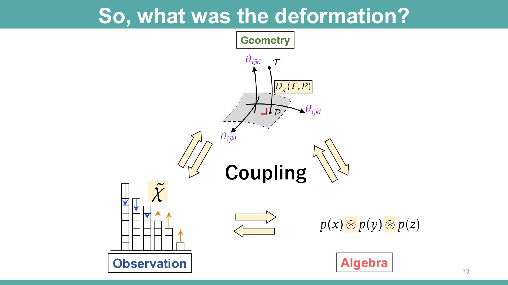
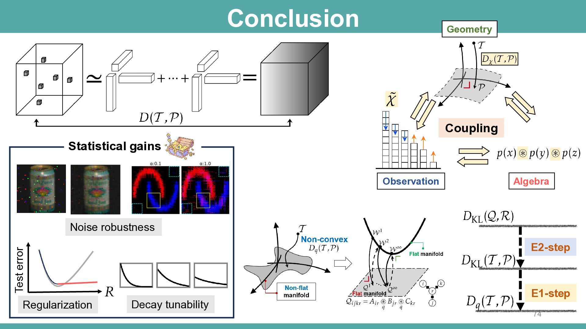
  69. Conclusion +⋯+ Geometry = Coupling Statistical gains Observation Algebra Noise

    robustness Test error E2-step Regularization Decay tunability E1-step 74
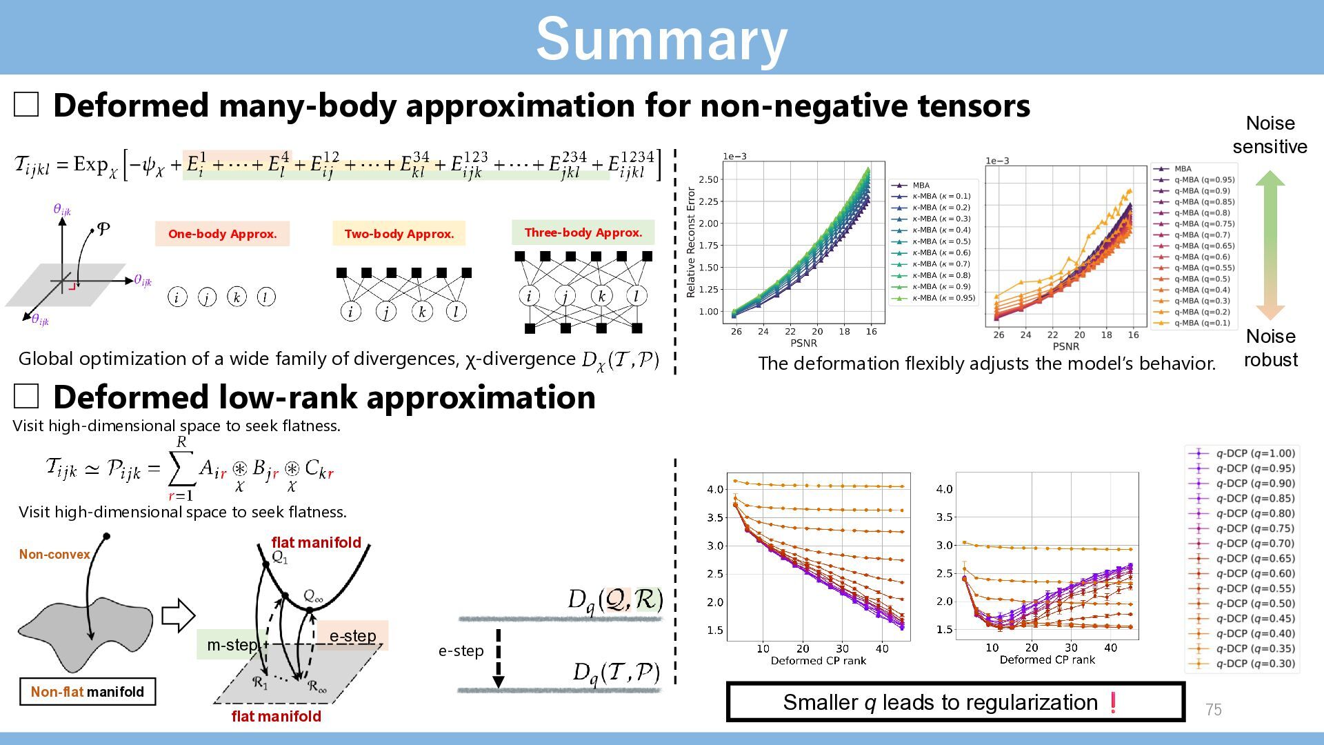
  70. Summary □ Deformed many-body approximation for non-negative tensors Two-body Approx.

    One-body Approx. Noise sensitive Three-body Approx. Global optimization of a wide family of divergences, χ-divergence □ Deformed low-rank approximation The deformation flexibly adjusts the model’s behavior. Visit high-dimensional space to seek flatness. Visit high-dimensional space to seek flatness. flat manifold Non-convex m-step Non-flat manifold flat manifold e-step e-step Smaller q leads to regularization 75 Noise robust