Analyzing cultural evolution with bayesian inference
Index
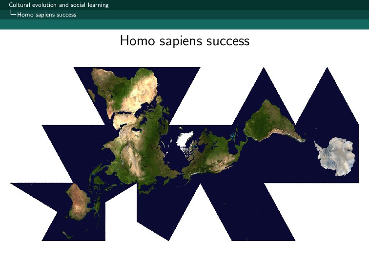
1- Why social learning is essential for human adaptation?
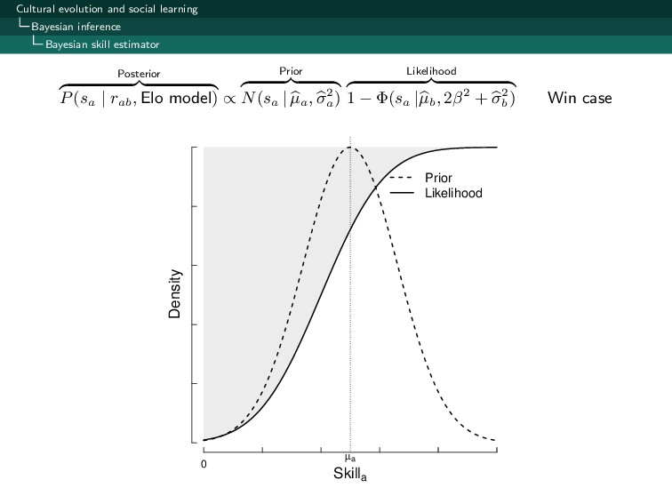
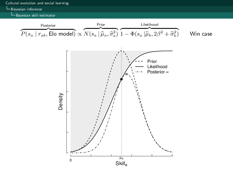
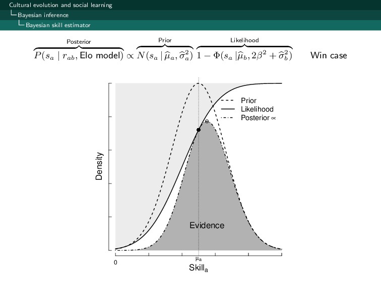
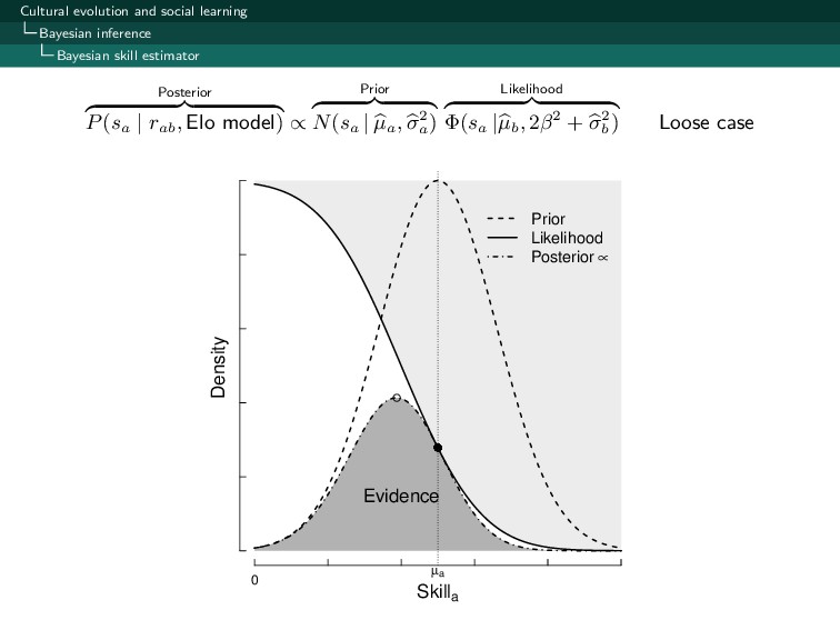
2- Why Bayesian inference allow us to estimate skill acquisition?
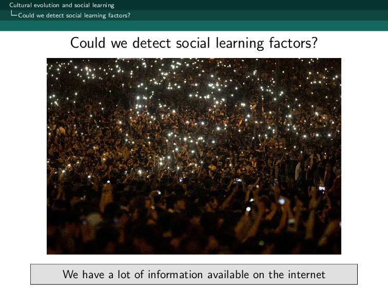
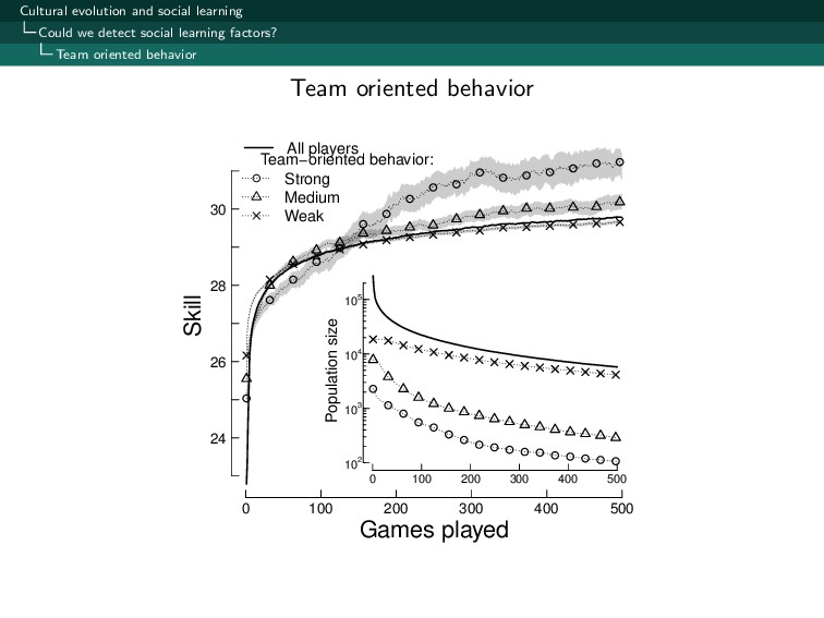
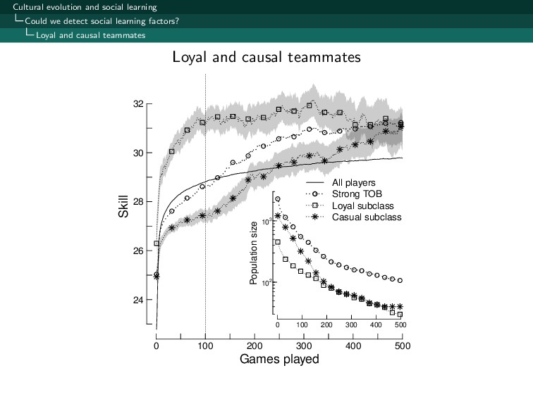
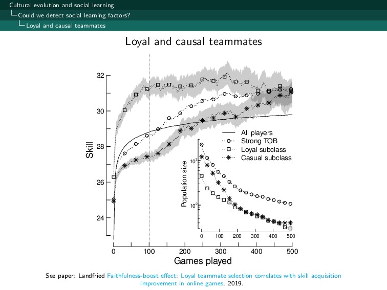
3- Could we detect social learning factors on an online game?
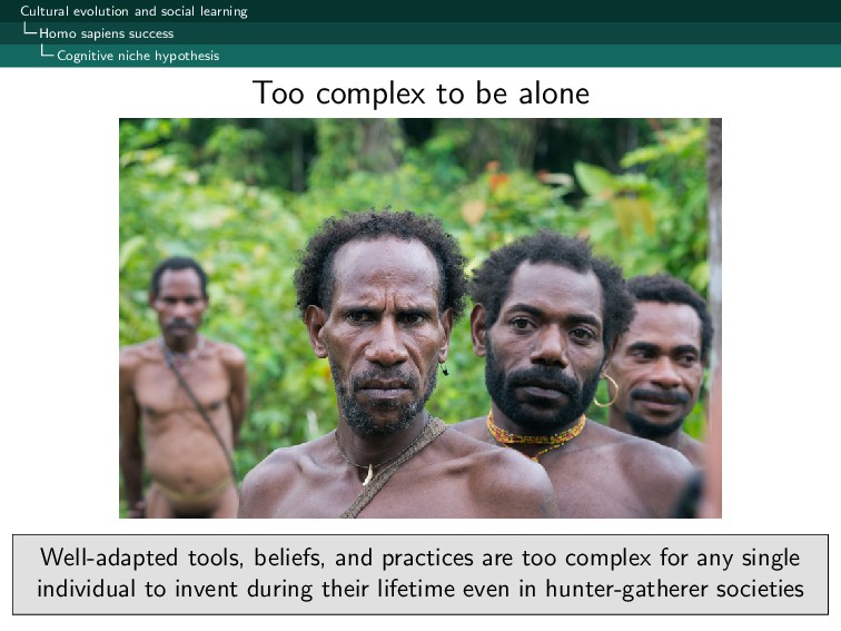
hypothesis Well-adapted tools, beliefs, and practices are too complex for any single individual to invent during their lifetime even in hunter-gatherer societies Too complex to be alone
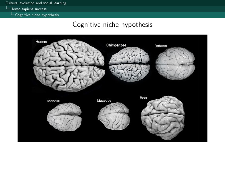
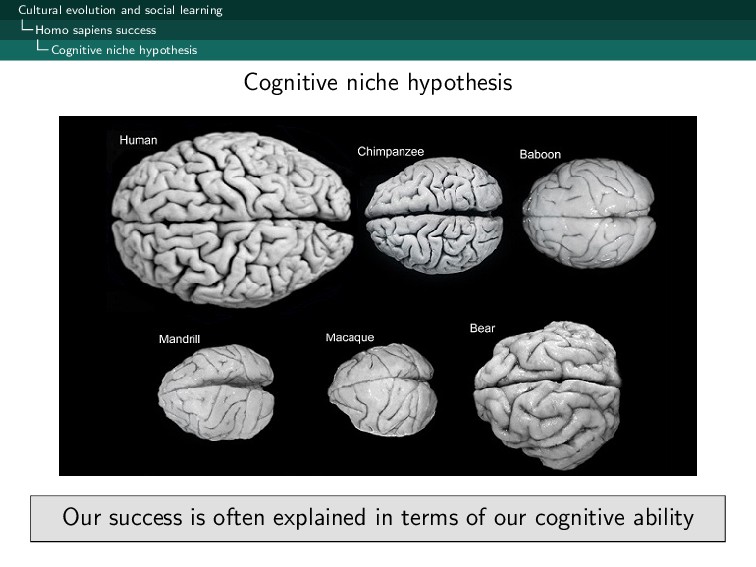
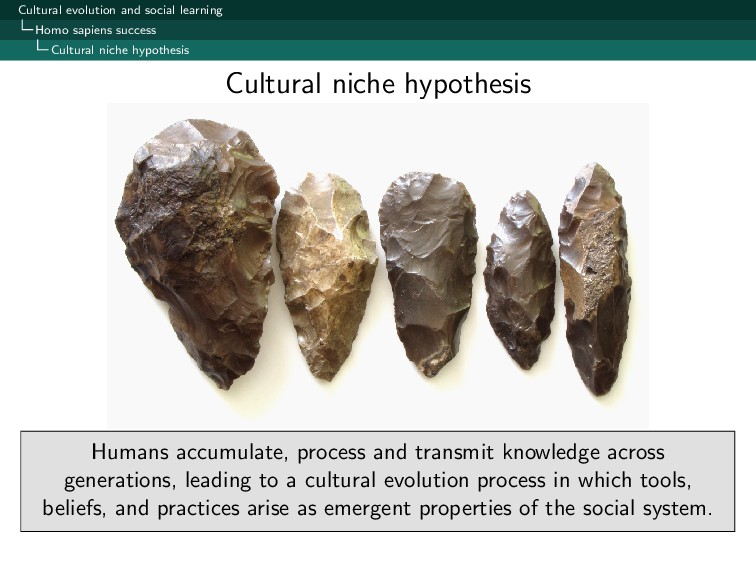
hypothesis Humans accumulate, process and transmit knowledge across generations, leading to a cultural evolution process in which tools, beliefs, and practices arise as emergent properties of the social system. Cultural niche hypothesis
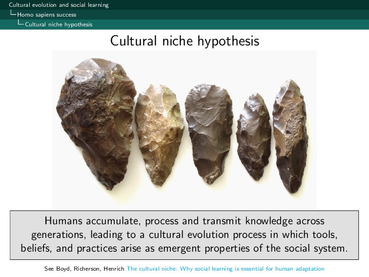
hypothesis Humans accumulate, process and transmit knowledge across generations, leading to a cultural evolution process in which tools, beliefs, and practices arise as emergent properties of the social system. See Boyd, Richerson, Henrich The cultural niche: Why social learning is essential for human adaptation Cultural niche hypothesis
We owe our success to our ability to learn from others (social learning) Books: Culture and the Evolutionary Process – Origine and Evolution of Cultures – Mathematical Models of Social Evolution. Cultural evolution
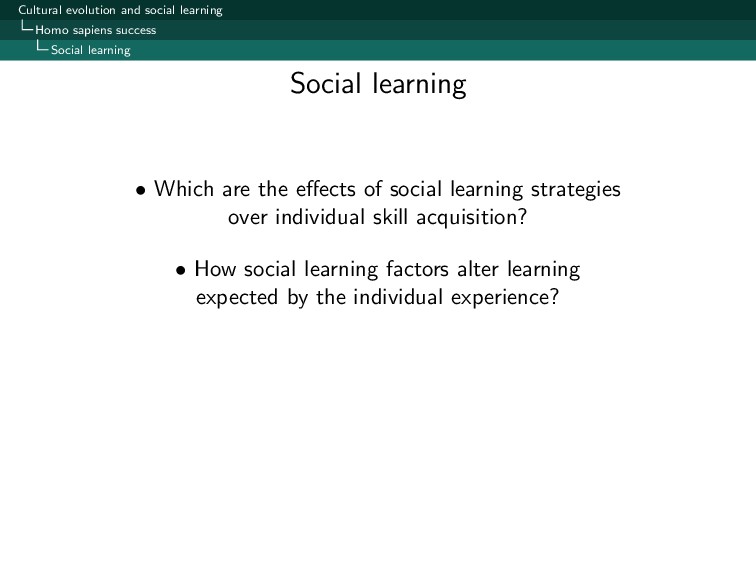
• Which are the effects of social learning strategies over individual skill acquisition? • How social learning factors alter learning expected by the individual experience? Social learning
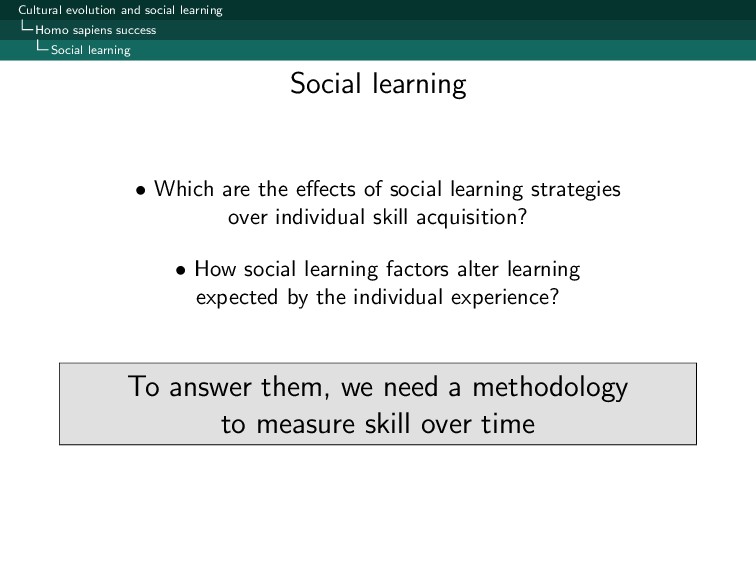
• Which are the effects of social learning strategies over individual skill acquisition? • How social learning factors alter learning expected by the individual experience? To answer them, we need a methodology to measure skill over time Social learning
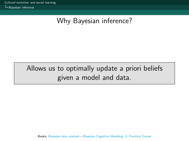
optimally update a priori beliefs given a model and data. Why Bayesian inference? Books: Bayesian data analysis – Bayesian Cognitive Modeling: A Practical Course
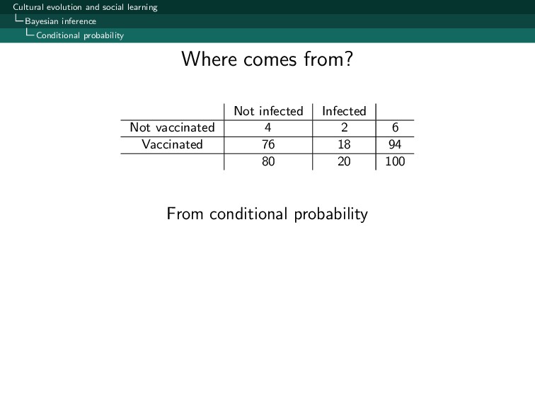
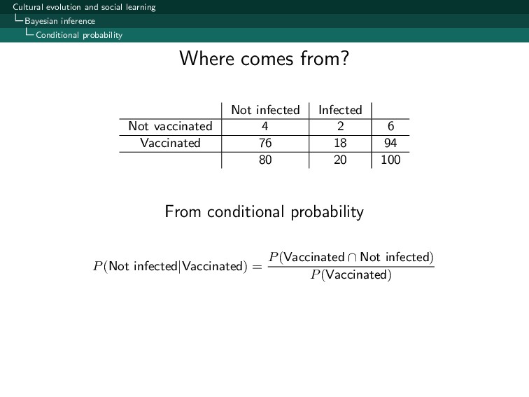
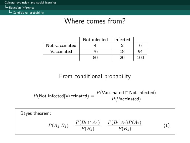
infected Infected Not vaccinated 4 2 6 Vaccinated 76 18 94 80 20 100 From conditional probability P(Not infected|Vaccinated) = P(Vaccinated ∩ Not infected) P(Vaccinated) Where comes from?
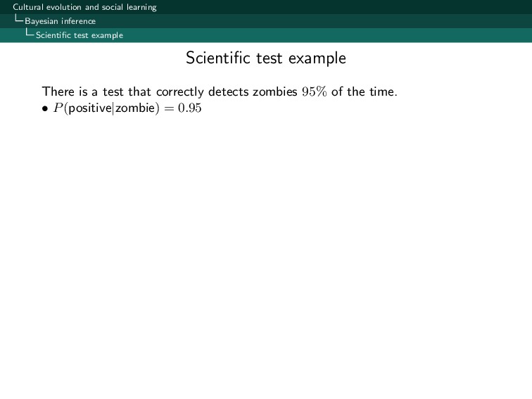
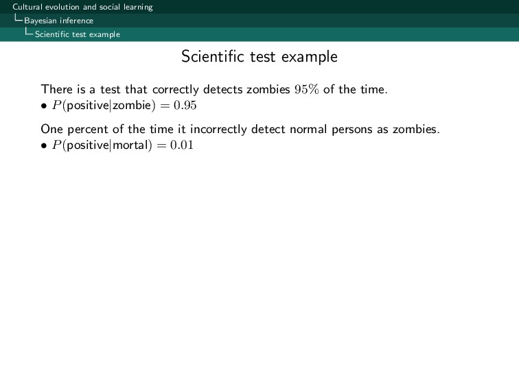
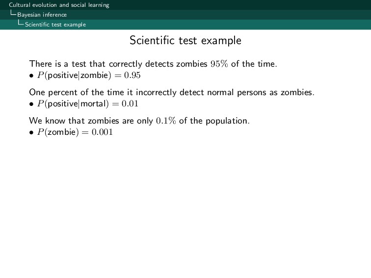
There is a test that correctly detects zombies 95% of the time. • P(positive|zombie) = 0.95 One percent of the time it incorrectly detect normal persons as zombies. • P(positive|mortal) = 0.01 Scientific test example
There is a test that correctly detects zombies 95% of the time. • P(positive|zombie) = 0.95 One percent of the time it incorrectly detect normal persons as zombies. • P(positive|mortal) = 0.01 We know that zombies are only 0.1% of the population. • P(zombie) = 0.001 Scientific test example
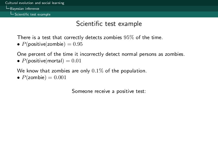
There is a test that correctly detects zombies 95% of the time. • P(positive|zombie) = 0.95 One percent of the time it incorrectly detect normal persons as zombies. • P(positive|mortal) = 0.01 We know that zombies are only 0.1% of the population. • P(zombie) = 0.001 Someone receive a positive test: Scientific test example
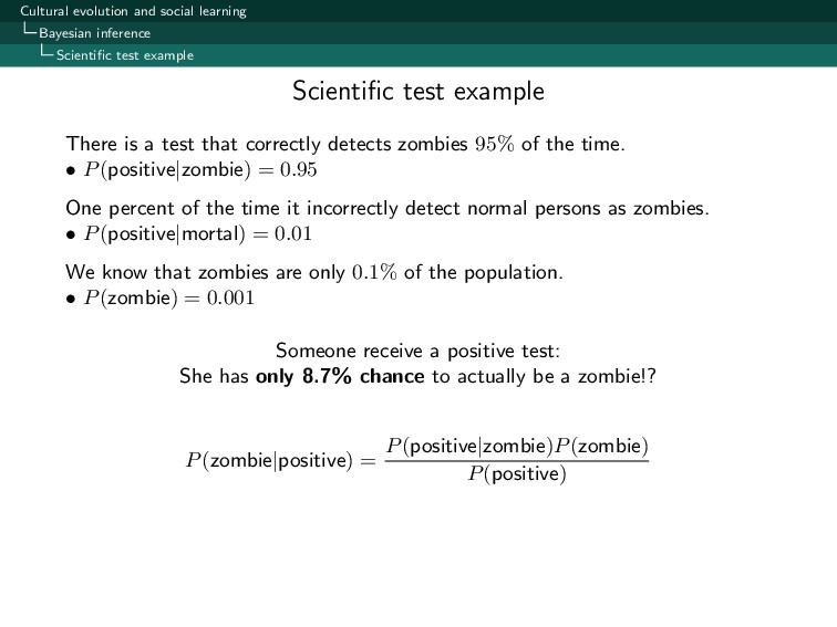
There is a test that correctly detects zombies 95% of the time. • P(positive|zombie) = 0.95 One percent of the time it incorrectly detect normal persons as zombies. • P(positive|mortal) = 0.01 We know that zombies are only 0.1% of the population. • P(zombie) = 0.001 Someone receive a positive test: She has only 8.7% chance to actually be a zombie!? P(zombie|positive) = P(positive|zombie)P(zombie) P(positive) Scientific test example
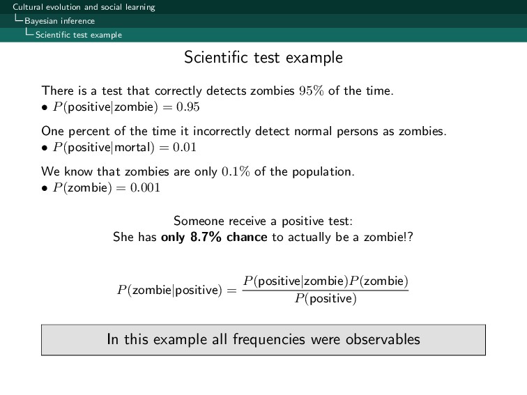
There is a test that correctly detects zombies 95% of the time. • P(positive|zombie) = 0.95 One percent of the time it incorrectly detect normal persons as zombies. • P(positive|mortal) = 0.01 We know that zombies are only 0.1% of the population. • P(zombie) = 0.001 Someone receive a positive test: She has only 8.7% chance to actually be a zombie!? P(zombie|positive) = P(positive|zombie)P(zombie) P(positive) In this example all frequencies were observables Scientific test example
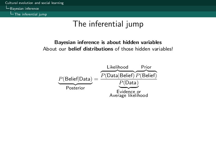
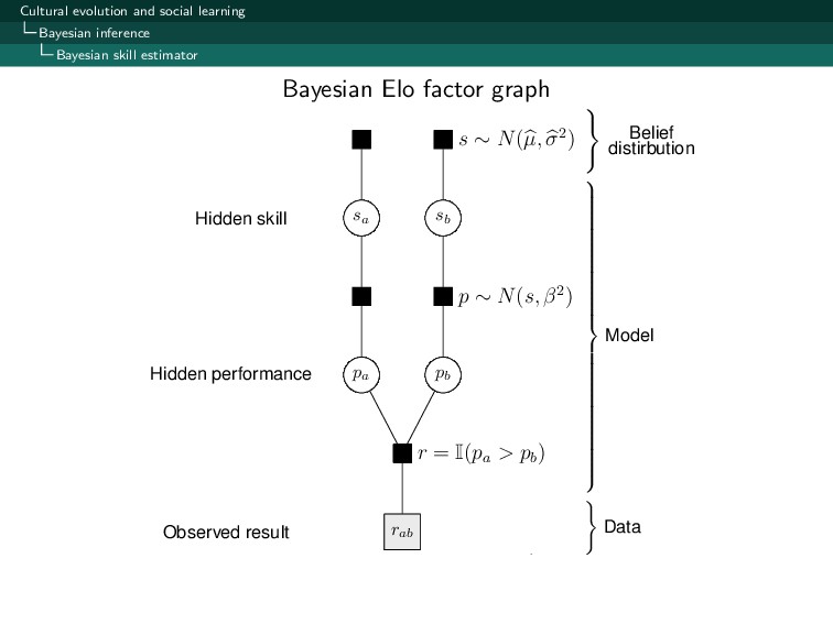
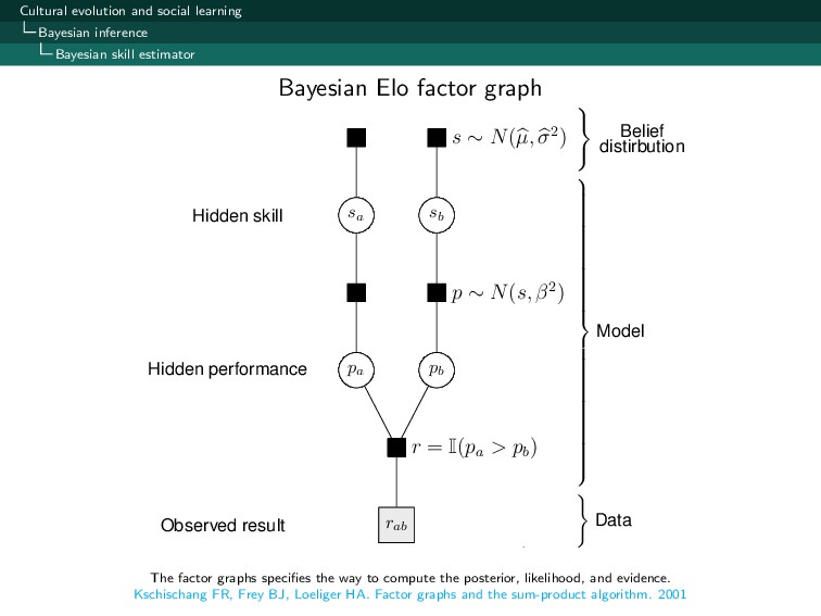
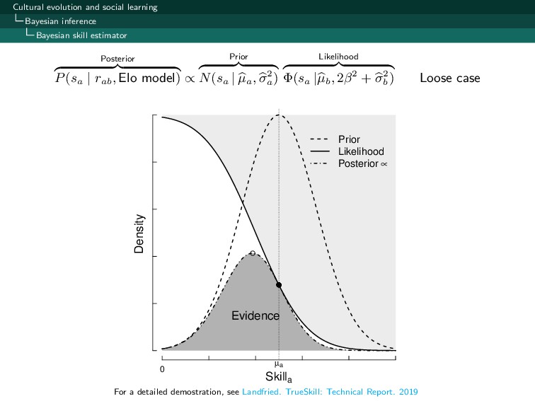
Bayesian inference is about hidden variables About our belief distributions of those hidden variables! P(Belief|Data) Posterior = Likelihood P(Data|Belief) Prior P(Belief) P(Data) Evidence or Average likelihood The inferential jump
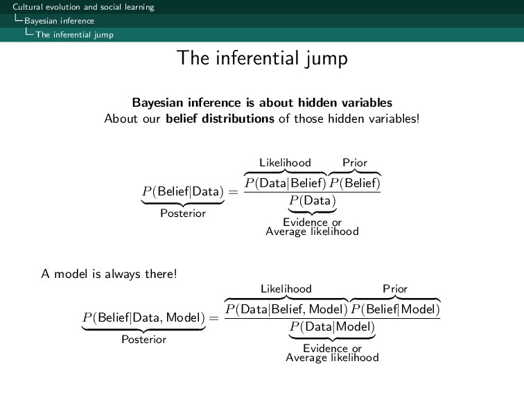
Bayesian inference is about hidden variables About our belief distributions of those hidden variables! P(Belief|Data) Posterior = Likelihood P(Data|Belief) Prior P(Belief) P(Data) Evidence or Average likelihood A model is always there! P(Belief|Data, Model) Posterior = Likelihood P(Data|Belief, Model) Prior P(Belief|Model) P(Data|Model) Evidence or Average likelihood The inferential jump
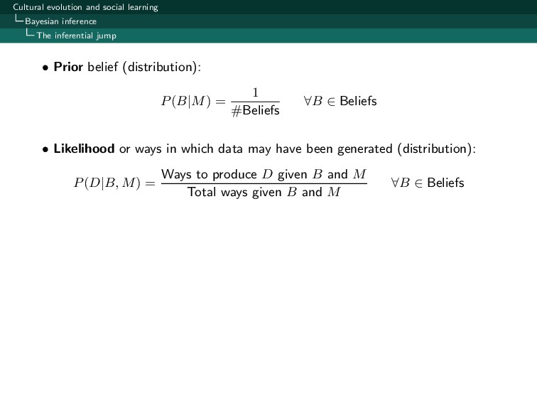
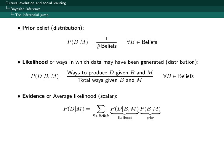
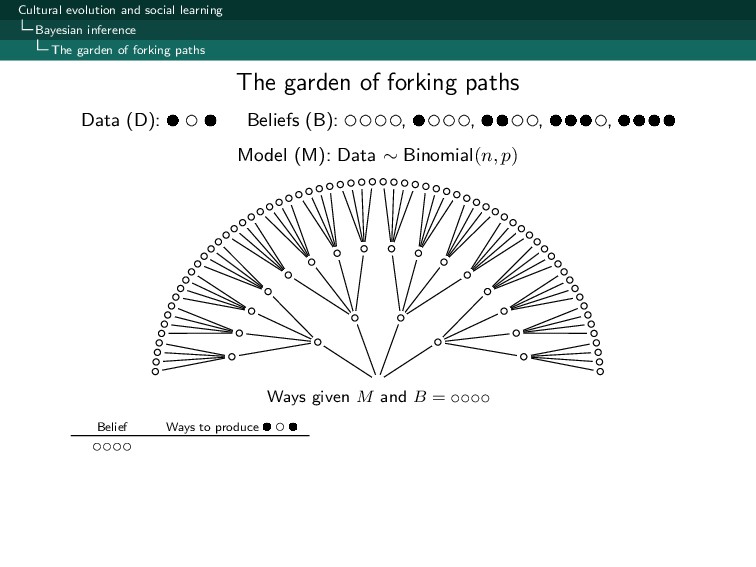
• Prior belief (distribution): P(B|M) = 1 #Beliefs ∀B ∈ Beliefs • Likelihood or ways in which data may have been generated (distribution): P(D|B, M) = Ways to produce D given B and M Total ways given B and M ∀B ∈ Beliefs
• Prior belief (distribution): P(B|M) = 1 #Beliefs ∀B ∈ Beliefs • Likelihood or ways in which data may have been generated (distribution): P(D|B, M) = Ways to produce D given B and M Total ways given B and M ∀B ∈ Beliefs • Evidence or Average likelihood (scalar): P(D|M) = B∈Beliefs P(D|B, M) likelihood P(B|M) prior
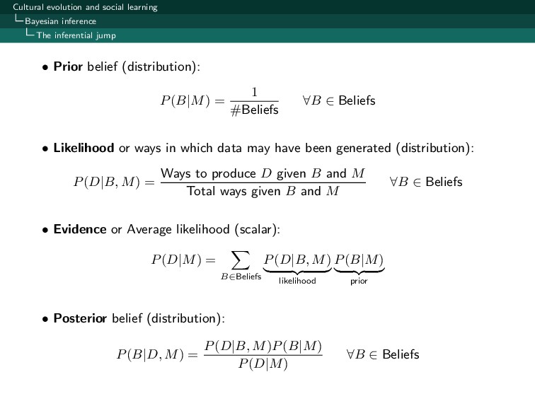
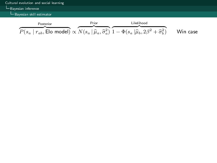
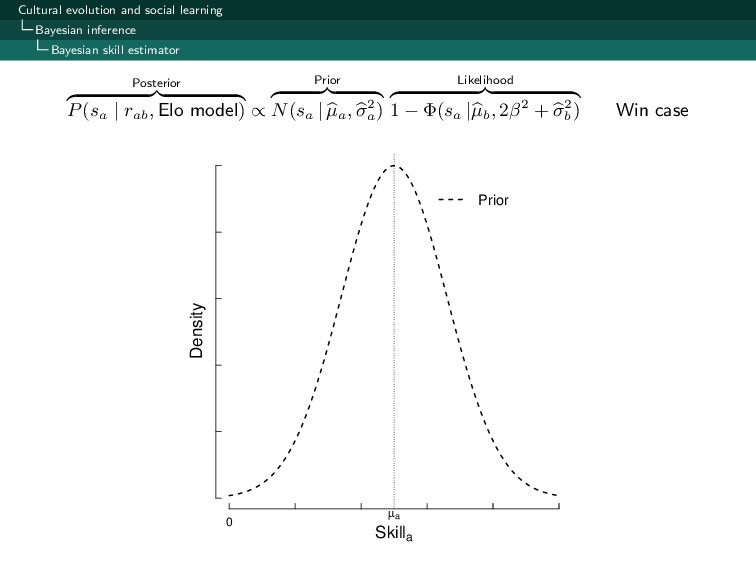
• Prior belief (distribution): P(B|M) = 1 #Beliefs ∀B ∈ Beliefs • Likelihood or ways in which data may have been generated (distribution): P(D|B, M) = Ways to produce D given B and M Total ways given B and M ∀B ∈ Beliefs • Evidence or Average likelihood (scalar): P(D|M) = B∈Beliefs P(D|B, M) likelihood P(B|M) prior • Posterior belief (distribution): P(B|D, M) = P(D|B, M)P(B|M) P(D|M) ∀B ∈ Beliefs
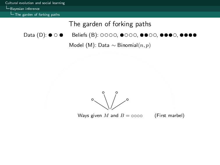
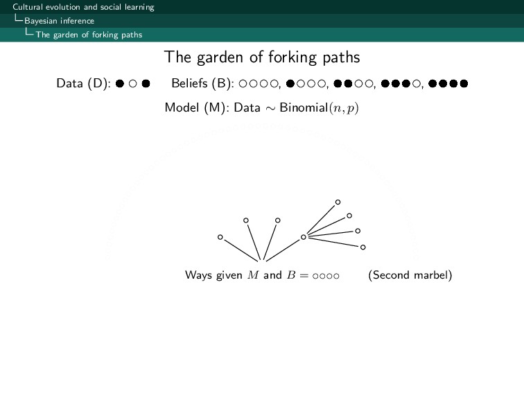
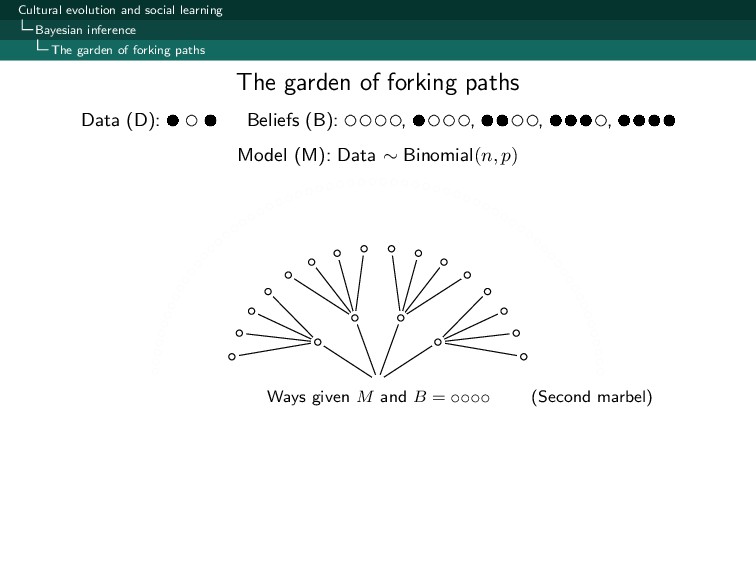
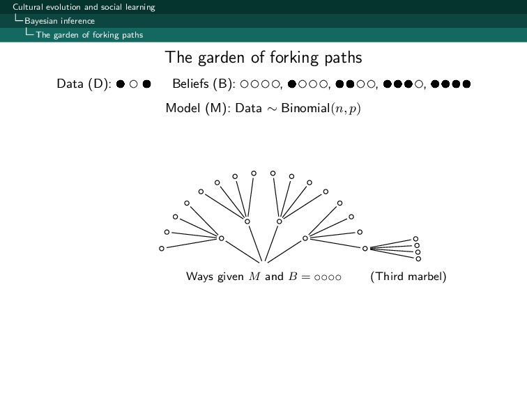
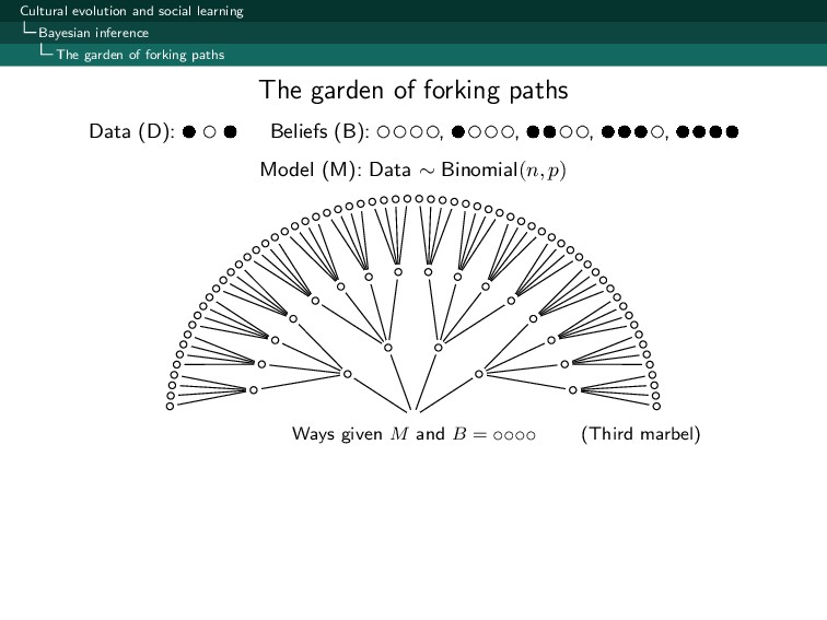
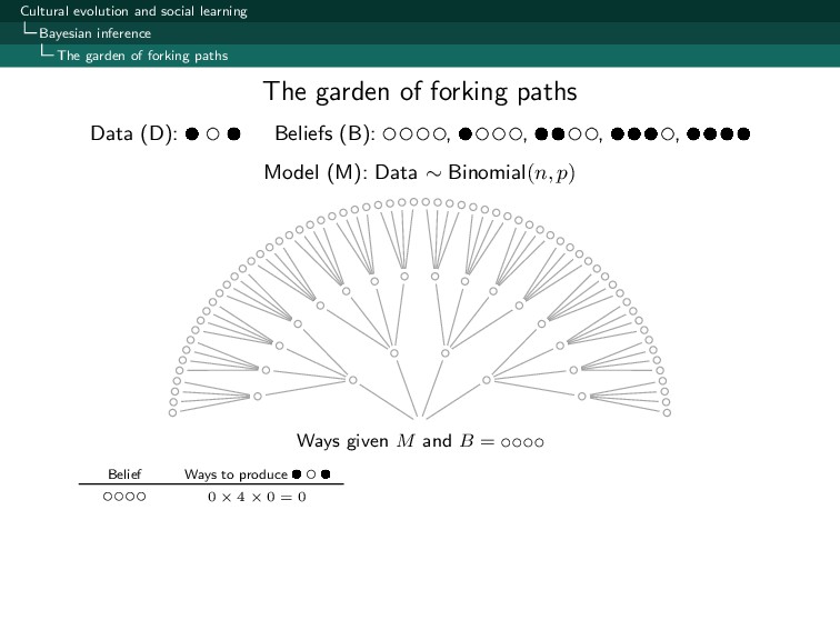
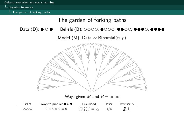
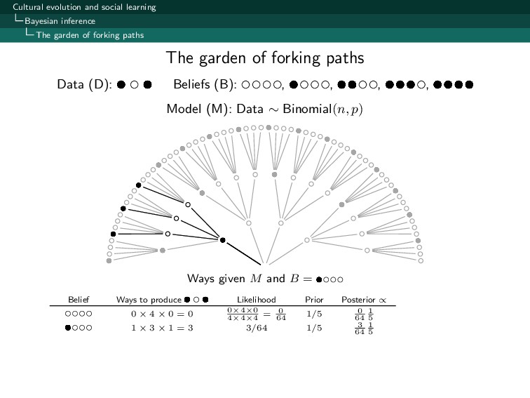
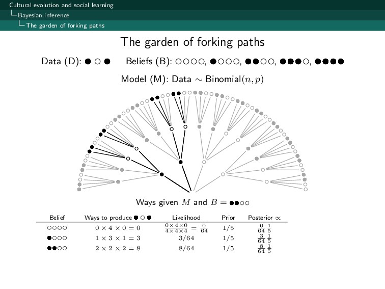
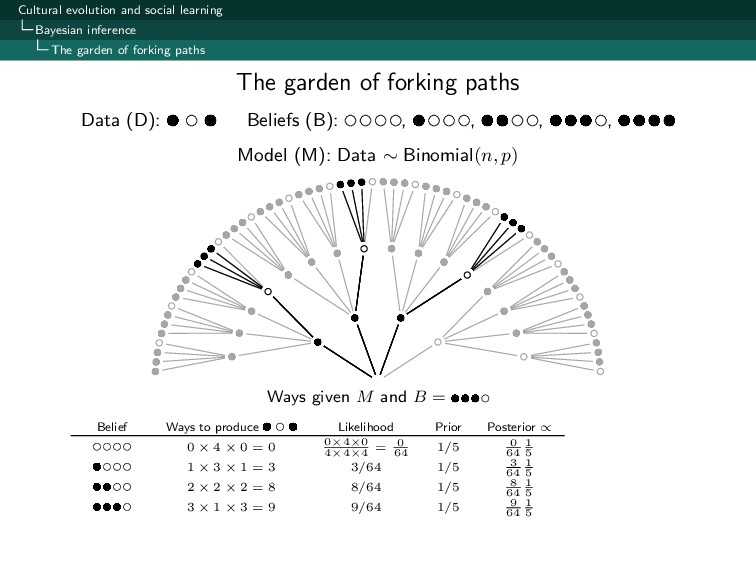
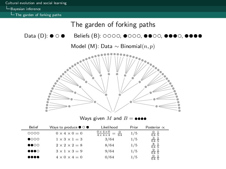
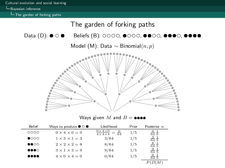
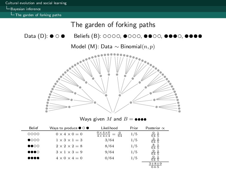
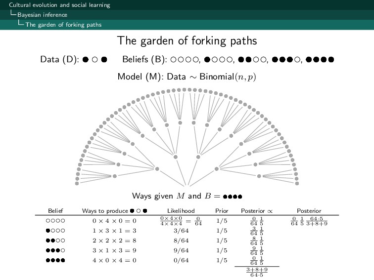
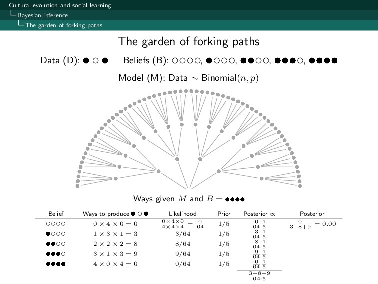
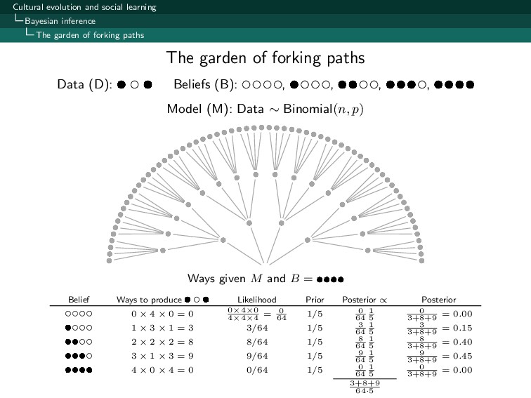
forking paths To update our beliefs (posterior), we need to consider every possible path in the model that could have lead us to the observed data (likelihood). The garden of forking paths
forking paths The garden of forking paths Data (D): Beliefs (B): , , , , Model (M): Data ∼ Binomial(n, p) (First marbel) q q q q q q q q q Ways given M and B =
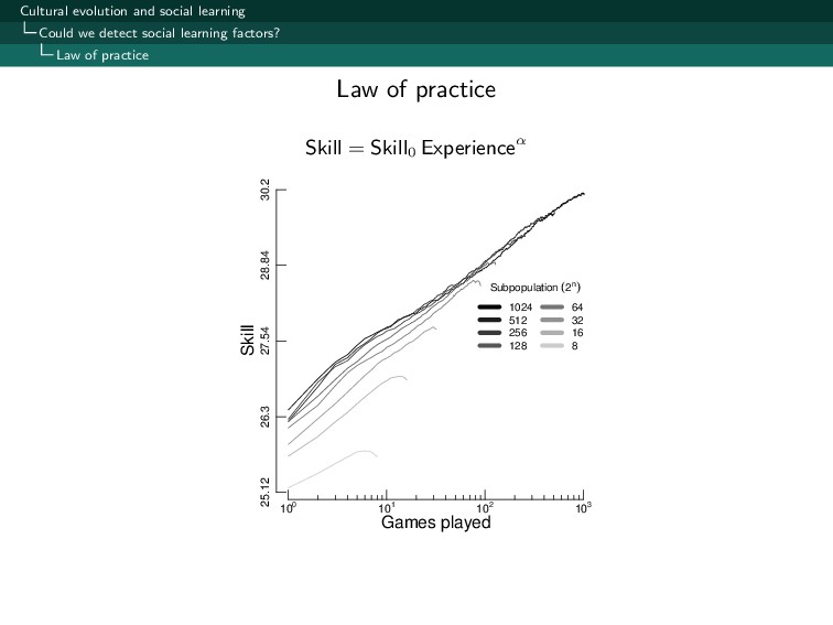
factors? Law of practice Skill = Skill0 Experienceα 100 101 102 103 25.12 26.3 27.54 28.84 30.2 Games played Skill Subpopulation (2n) 1024 512 256 128 64 32 16 8 Law of practice
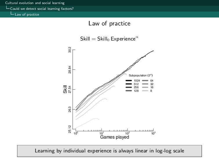
factors? Law of practice Skill = Skill0 Experienceα 100 101 102 103 25.12 26.3 27.54 28.84 30.2 Games played Skill Subpopulation (2n) 1024 512 256 128 64 32 16 8 Learning by individual experience is always linear in log-log scale Law of practice