Measuring fundamental properties of young stars

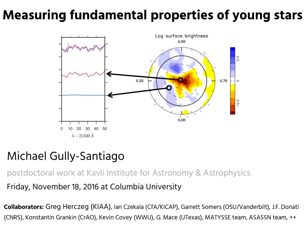
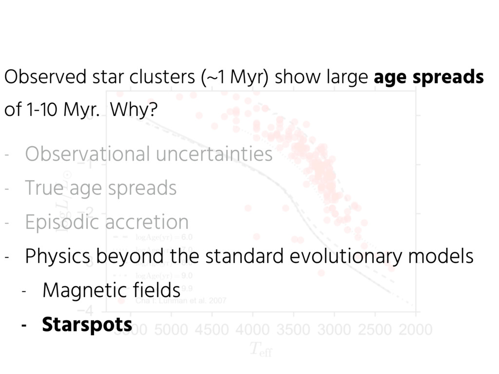
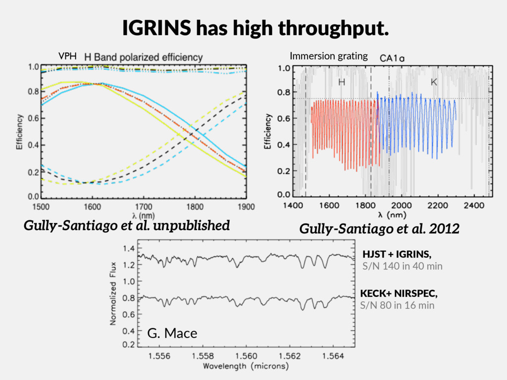
Talk at Columbia University Stellar and Planetary lunch talk on Friday, November 18, 2016. Hosted by Stephanie Douglas.

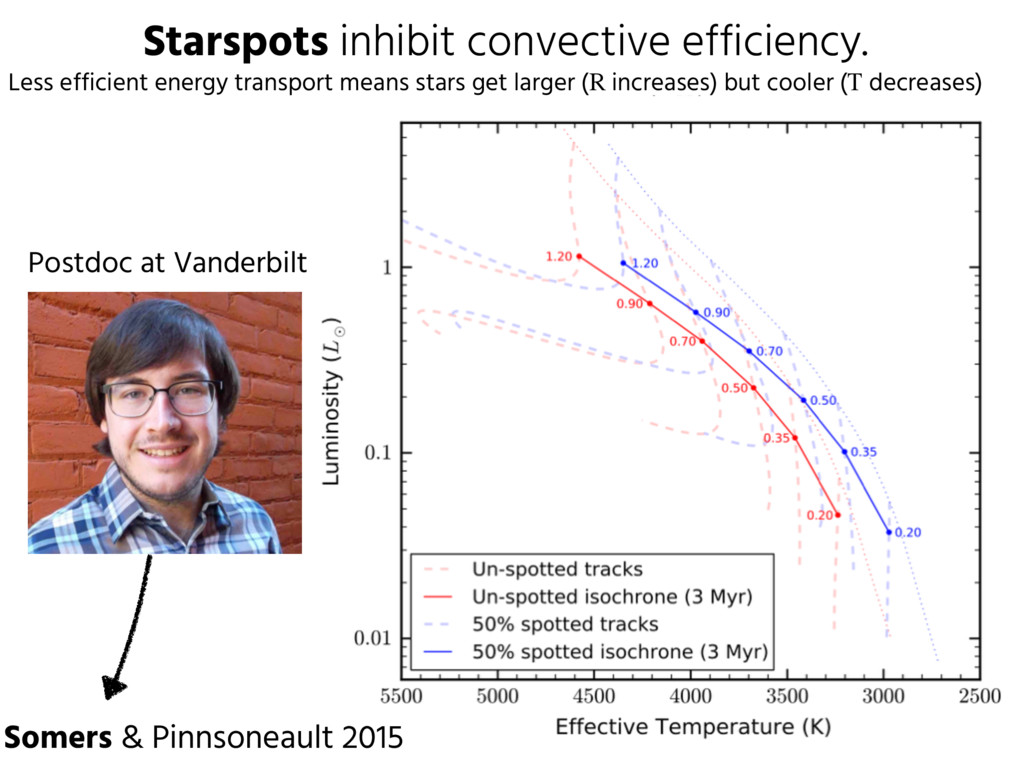
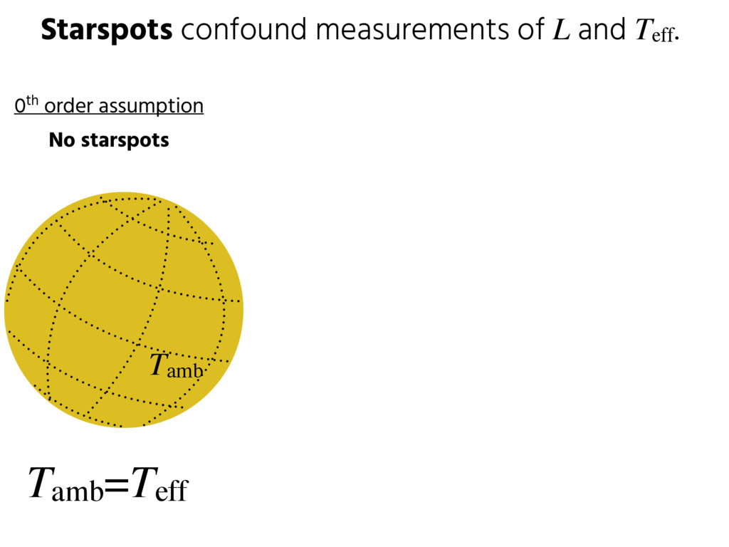
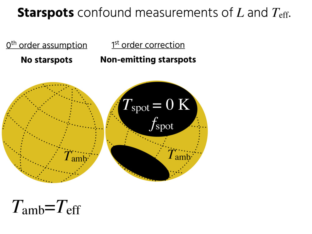
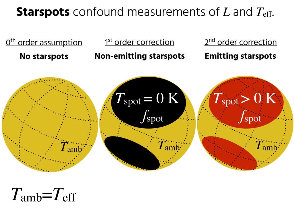
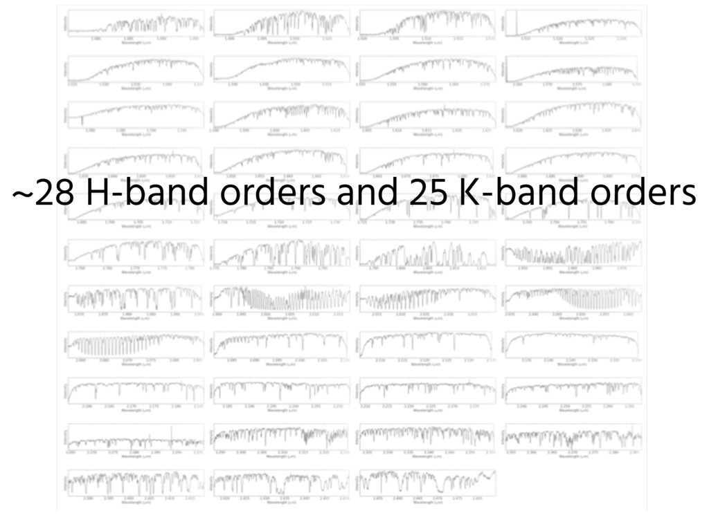
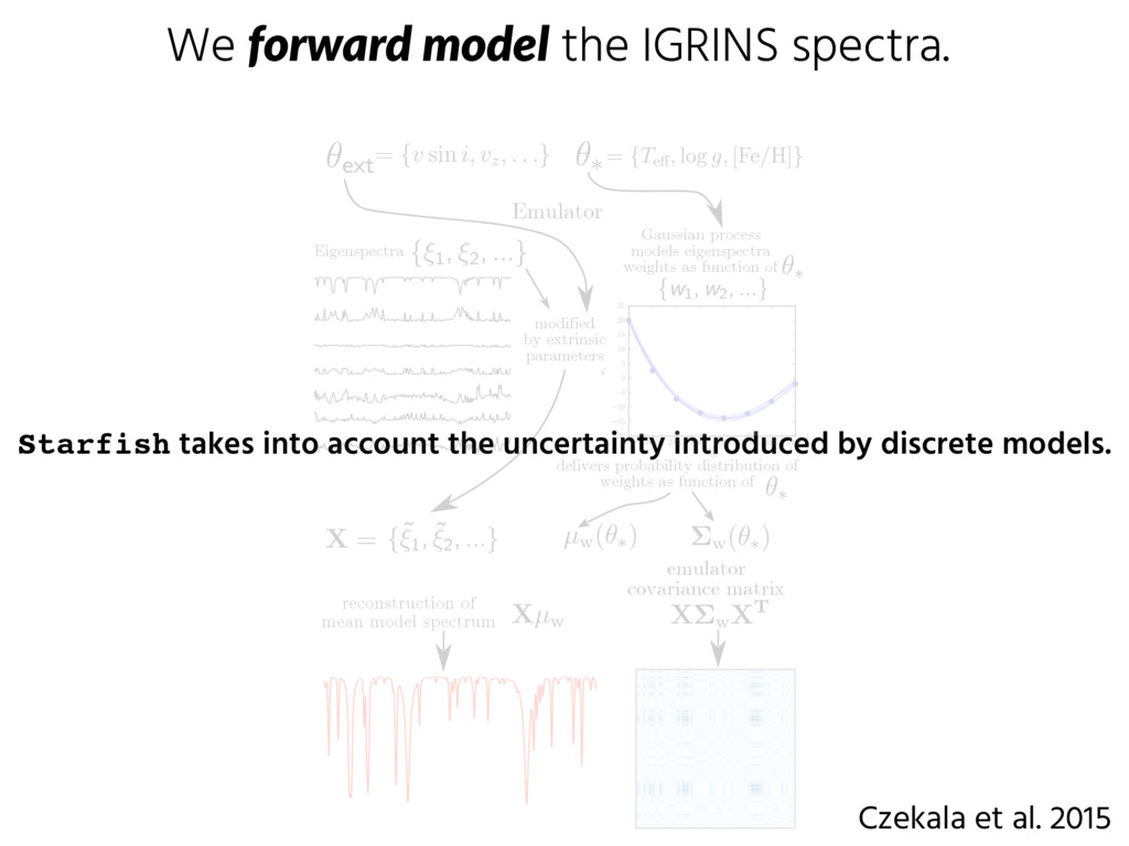
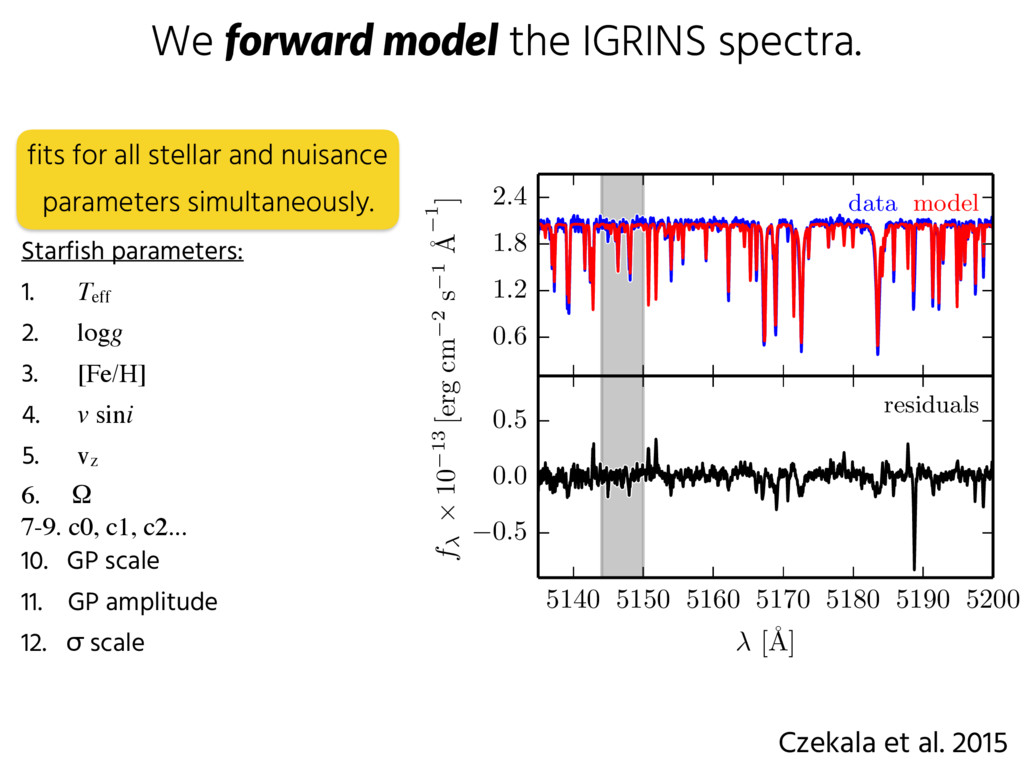
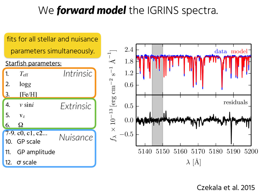
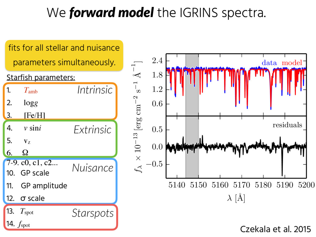
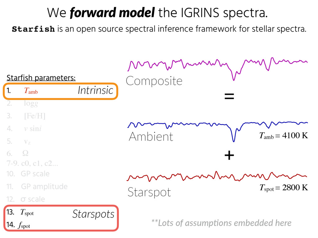
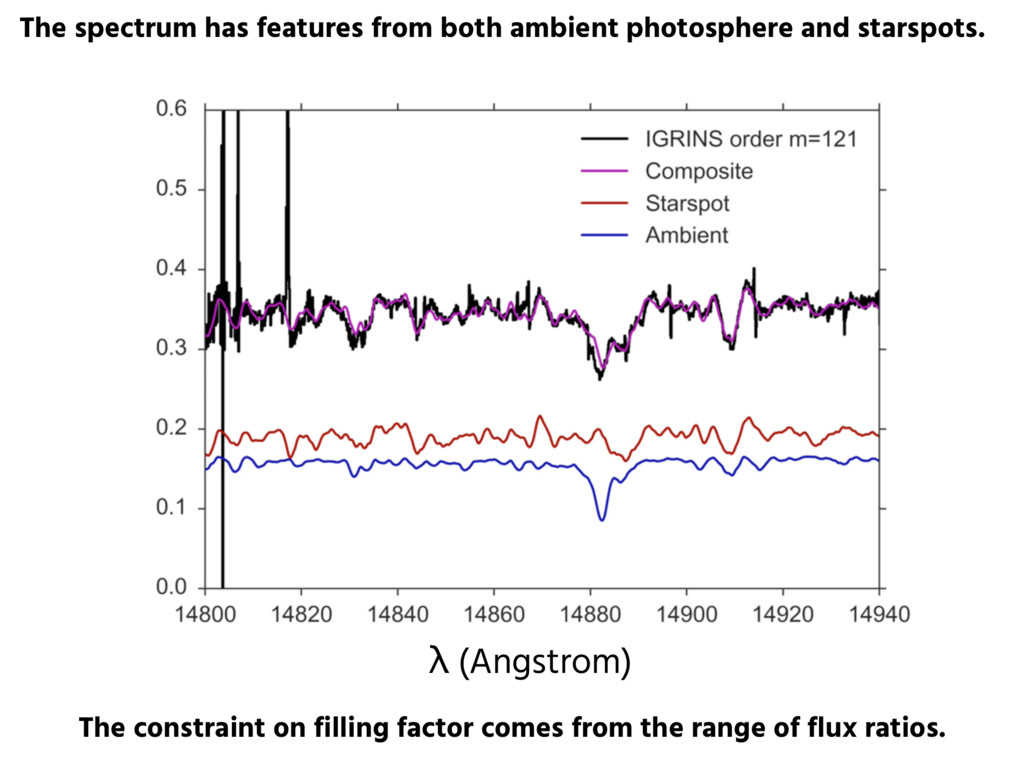
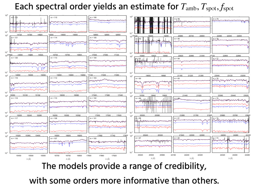
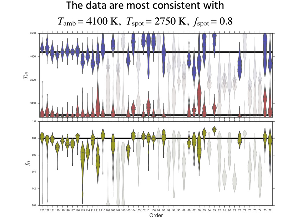
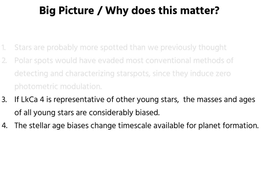
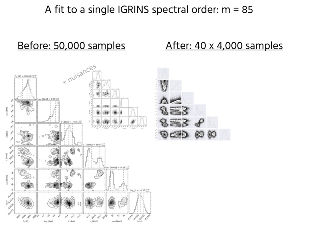
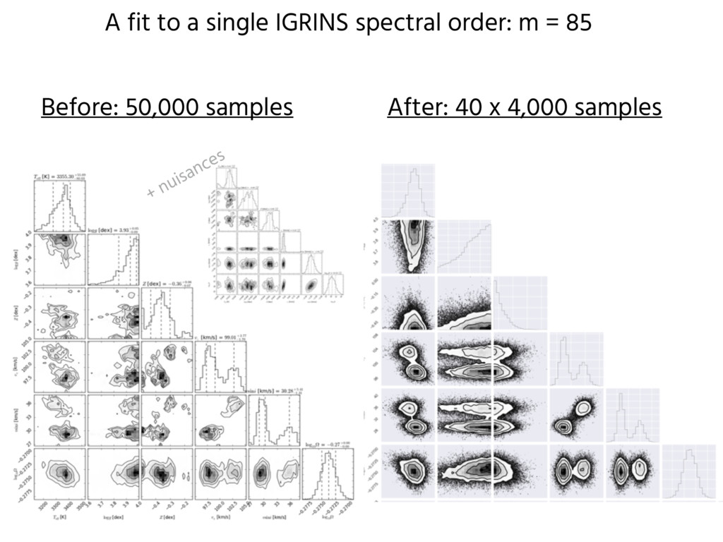
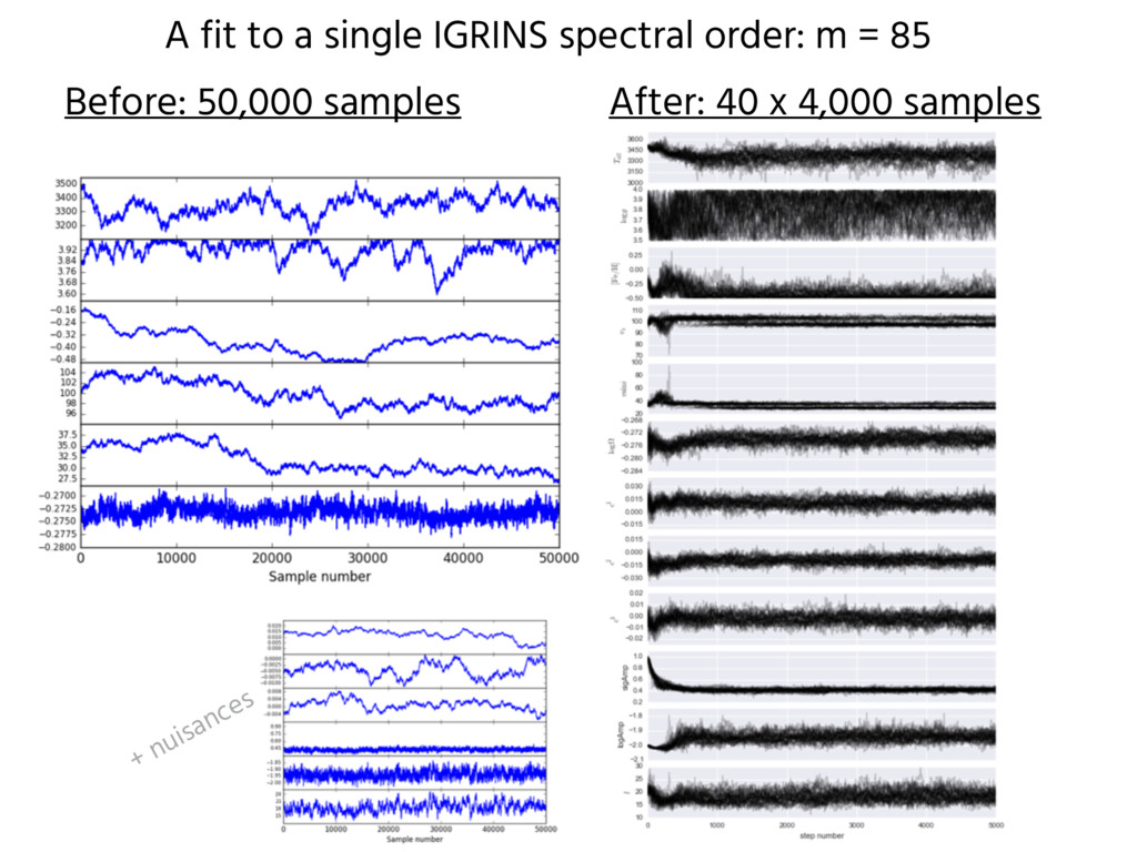
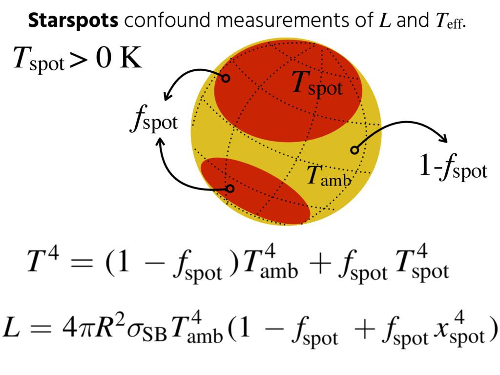
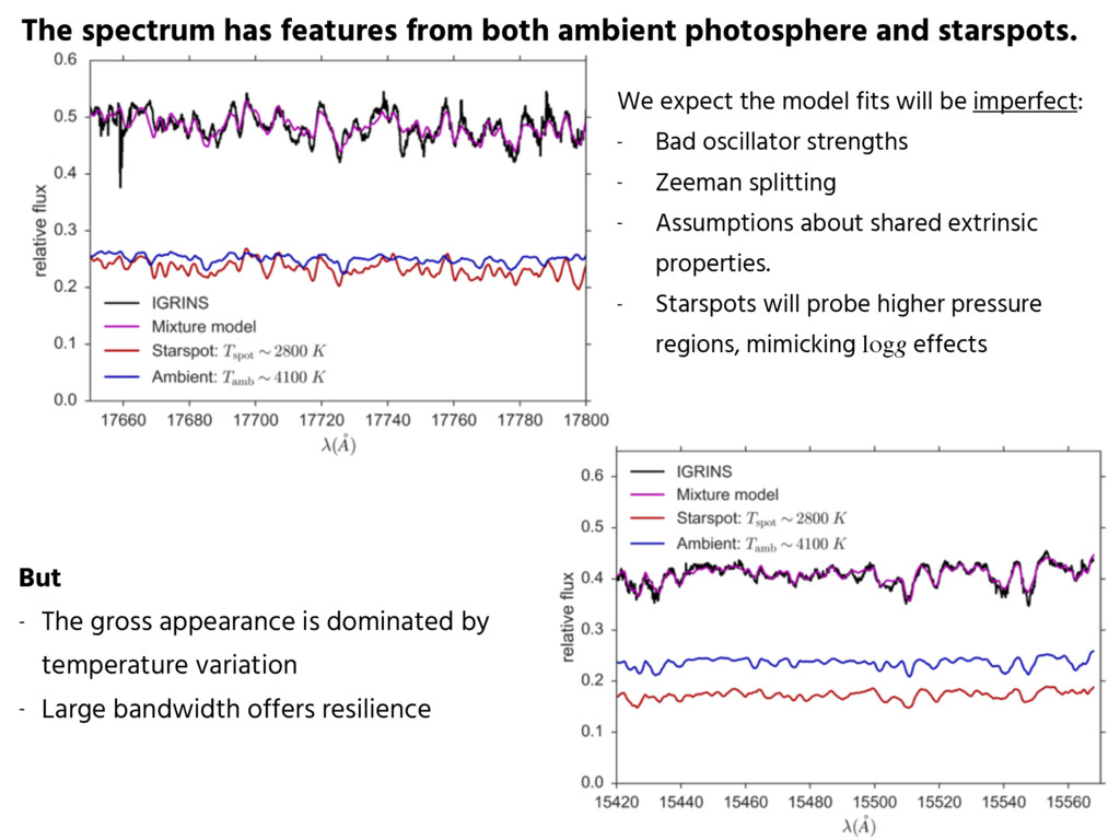
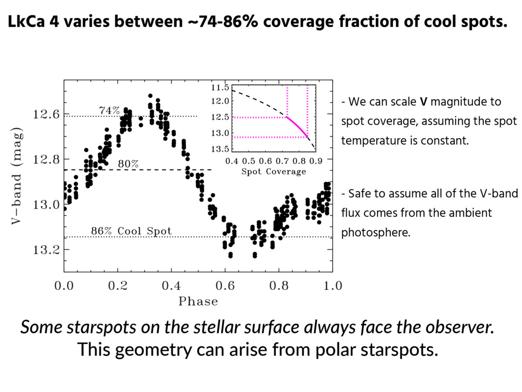
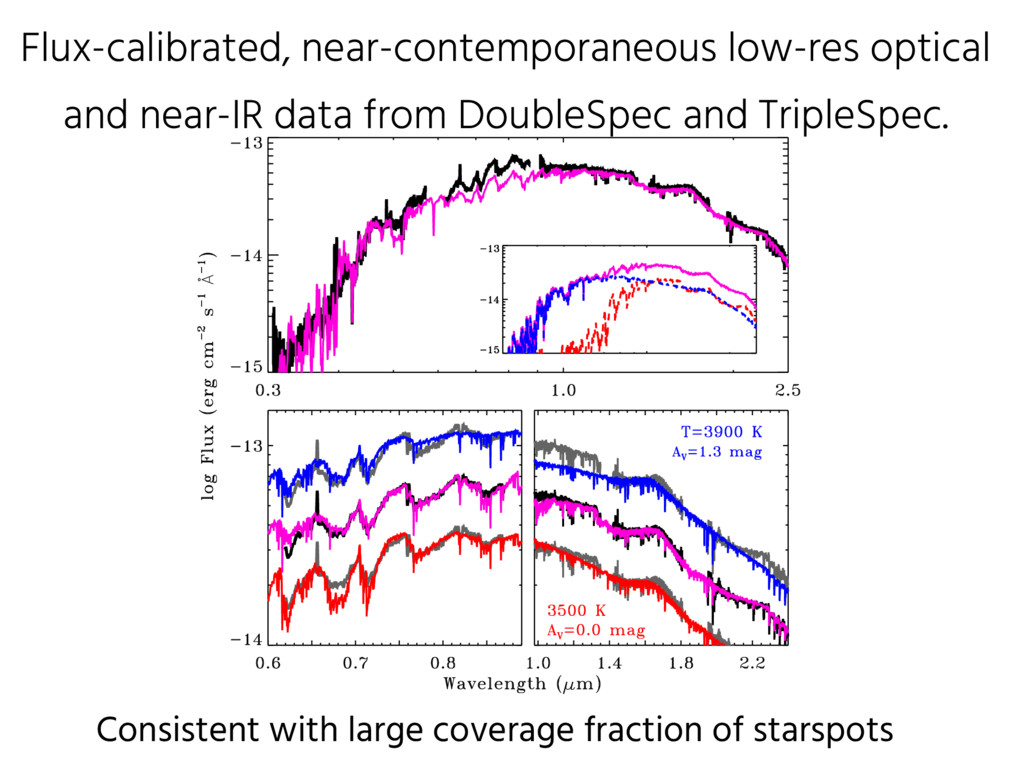
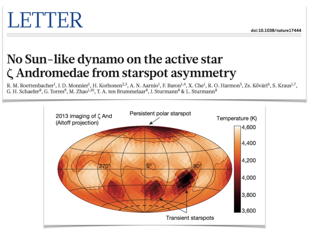
We measured the starspot temperature and coverage fraction using IGRINS spectra and spectroscopic inference. Starspots are a confounding factor in assigning temperatures and therefore ages to young stars.

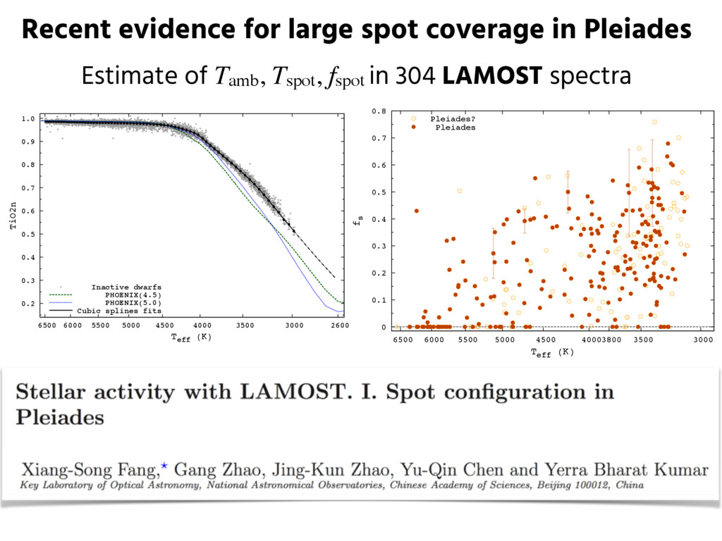
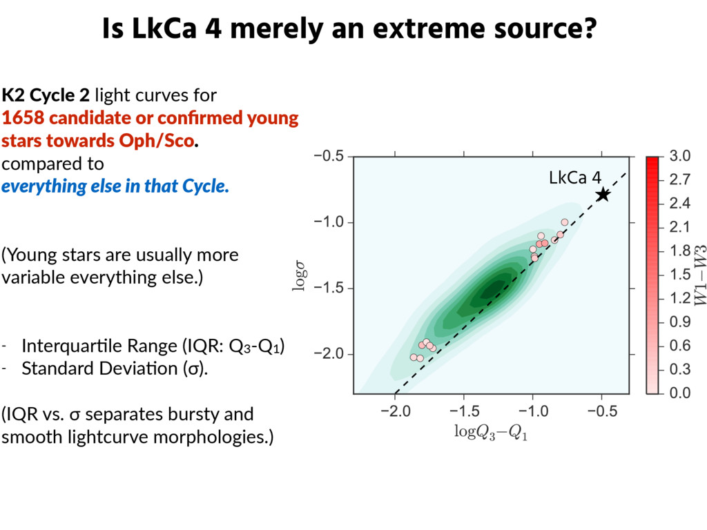
The Figure on Slide 42 has been updated with revised calculations, please see the arXiv paper or ApJ paper for the most up-to-date, downloadable figures and data.

Transcript

1. Measuring fundamental properties of young stars
   Michael Gully-Santiago
   postdoctoral work at Kavli Institute for Astronomy & Astrophysics
   Friday, November 18, 2016 at Columbia University
   Collaborators: Greg Herczeg (KIAA), Ian Czekala (CfA/KICAP), Garrett Somers (OSU/Vanderbilt), J.F. Donati
   (CNRS), Konstantin Grankin (CrAO), Kevin Covey (WWU), G. Mace (UTexas), MATYSSE team, ASASSN team, ++
   

   View Slide

2. We want to know the ages and masses of young
   stars so that we can understand how star and planet
   formation proceed in time.
   

   View Slide

3. We want to know the ages and masses of young
   stars so that we can understand how star and planet
   formation proceed in time.
   Age is not a direct observable. Mass is sometimes a
   direct observable, but only in rare eclipsing binary
   systems or resolved gas disk systems.
   

   View Slide

4. Ages are estimated by placing a young star on a pre-main sequence HR diagram.
   

   View Slide

5. Ages are estimated by placing a young star on a pre-main sequence HR diagram.
   

   View Slide

6. Observed star clusters (~1 Myr) show large age spreads
   of 1-10 Myr. Why?
   

   View Slide

7. Observed star clusters (~1 Myr) show large age spreads
   of 1-10 Myr. Why?
   - Observational uncertainties
   - True age spreads
   - Episodic accretion
   - Physics beyond the standard evolutionary models
   - Magnetic fields
   - Starspots
   

   View Slide

8. Observed star clusters (~1 Myr) show large age spreads
   of 1-10 Myr. Why?
   - Observational uncertainties
   - True age spreads
   - Episodic accretion
   - Physics beyond the standard evolutionary models
   - Magnetic fields
   - Starspots
   

   View Slide

9. Observed star clusters (~1 Myr) show large age spreads
   of 1-10 Myr. Why?
   - Observational uncertainties
   - True age spreads
   - Episodic accretion
   - Physics beyond the standard evolutionary models
   - Magnetic fields
   - Starspots
   

   View Slide

10. Observed star clusters (~1 Myr) show large age spreads
    of 1-10 Myr. Why?
    - Observational uncertainties
    - True age spreads
    - Episodic accretion
    - Physics beyond the standard evolutionary models
    - Magnetic fields
    - Starspots
    

    View Slide

11. Observed star clusters (~1 Myr) show large age spreads
    of 1-10 Myr. Why?
    - Observational uncertainties
    - True age spreads
    - Episodic accretion
    - Physics beyond the standard evolutionary models
    - Magnetic fields
    - Starspots
    

    View Slide

12. Starspots inhibit convective efficiency.
    Somers & Pinnsoneault 2015
    Less efficient energy transport means stars get larger (R increases) but cooler (T decreases)
    Postdoc at Vanderbilt
    

    View Slide

13. Starspots confound measurements of L and Teff.
    Tamb=Teff
    0th order assumption
    No starspots
    Tamb
    

    View Slide

14. Starspots confound measurements of L and Teff.
    Tamb=Teff
    0th order assumption
    No starspots
    1st order correction
    Non-emitting starspots
    Tamb
    Tspot = 0 K
    fspot
    Tamb
    

    View Slide

15. Starspots confound measurements of L and Teff.
    Tamb=Teff
    0th order assumption
    No starspots
    1st order correction
    Non-emitting starspots
    Tamb
    Tspot > 0 K
    fspot
    Tamb
    Tspot = 0 K
    fspot
    Tamb
    2nd order correction
    Emitting starspots
    

    View Slide

16. Starspots confound measurements of L and Teff.
    Tamb=Teff
    0th order assumption
    No starspots
    1st order correction
    Non-emitting starspots
    Tamb
    Tspot > 0 K
    fspot
    Tamb
    Tspot = 0 K
    fspot
    Tamb
    2nd order correction
    Emitting starspots
    Teff < Tamb
    

    View Slide

17. Starspots confound measurements of L and Teff.
    Tamb
    Tspot
    fspot
    1-fspot
    My Research
    - We directly detect the spectrum arising from starspots.
    - That should probably surprise you... T4 is steep!
    - Not only that, but starspots are on Wien side of BB curve.
    - We benefit from moving to the infrared and high res.
    - Still: You need large covering fraction of spots to make up for T4
    

    View Slide

18. Starspot emission
    Tamb
    Tspot
    fspot
    1-fspot
    Tspot = 2800 K
    Tamb = 4100 K
    fspot = 0.5 (!)
    Example
    Key insight:
    - In the visible, starspot flux is
    5-20x weaker than the ambient
    photosphere.
    - In the near-IR, starspot flux is
    only 2.5-4x weaker than ambient
    

    View Slide

19. Starspot emission
    Tamb
    Tspot
    fspot
    1-fspot
    Tspot = 2800 K
    Tamb = 4100 K
    fspot = 0.5 (!)
    Example
    Key insight:
    - In the visible, starspot flux is
    5-20x weaker than the ambient
    photosphere.
    - In the near-IR, starspot flux is
    only 2.5-4x weaker than ambient
    IGRINS
    ESPaDOnS
    

    View Slide

20. IGRINS:
    Immersion Grating Infrared Spectrograph
    Park et al. 2014
    - R = λ/δλ = 45,000
    - Δλ = 1.4 - 2.4 μm
    - 2.7 m HJST at McDonald Observatory (*now 4.3 m DCT at Lowell Observatory)
    - Single slit echelle spectrograph: ~28 H-band orders and 25 K-band orders
    Silicon Immersion Grating
    (diffraction grating)
    Gully-Santiago et al. 2012
    

    View Slide

21. ~28 H-band orders and 25 K-band orders
    

    View Slide

22. LkCa 4 is an ideal target for detecting starspot emission.
    Vrba et al. 1993
    1. Associated with nearby (~140 pc) Taurus
    young (~1 Myr) star cluster
    2. No mid-IR to sub-mm excess that would
    indicate a circumstellar disk
    3. Weak-lined T-Tauri Star (no ongoing
    accretion based on UV excess).
    4. No evidence for a nearby companion from
    AO imaging, and spec. monitoring
    5. Large amplitude of photometric variability
    6. Availability of >20 years of polychromatic
    photometric monitoring
    7. Recent spectropolarimetric tomography
    Hartigan+ 1995, Andrews & Williams 2005, Edwards+ 2006,
    Kraus+ 2011, Nguyen+ 2012, Donati+ 2014, Grankin+ 2008
    

    View Slide

23. LkCa 4 is an ideal target for detecting starspot emission.
    Vrba et al. 1993
    1. Associated with nearby (~140 pc) Taurus
    young (~1 Myr)
    2. No mid-IR to sub-mm excess that would
    indicate a circumstellar disk
    3. Weak-lined T-Tauri Star (no ongoing
    accretion based on UV excess).
    4. No evidence for a nearby companion from
    AO imaging, and spec. monitoring
    5. Large amplitude of photometric variability
    6. Availability of >20 years of polychromatic
    photometric monitoring
    7. Recent spectropolarimetric tomography
    Hartigan+ 1995, Andrews & Williams 2005, Edwards+ 2006,
    Kraus+ 2011, Nguyen+ 2012, Donati+ 2014, Grankin+ 2008
    LkCa 4 spectrum should be devoid of complicating factors,
    and should have a large starspot signal in its spectrum.
    

    View Slide

24. LkCa 4 spectrum should be devoid of complicating factors,
    and should have a large starspot signal in its spectrum.
    How to figure out which lines are attributable to
    starspots or ambient photosphere?
    portion of LkCa 4 IGRINS spectrum
    from November 2015
    

    View Slide

25. We forward  model the IGRINS spectra.
    0.0
    0.2
    0.4
    0.6
    0.8
    1.0 raw
    5164 5165 5166 5167 5168 5169 5170
    [˚
    A]
    0.0
    0.2
    0.4
    0.6
    0.8
    1.0 convolved and resampled
    f ⇥ 107 [erg cm 2 s 1 ˚
    A 1
    ]
    Synthetic spectra from pre-computed PHOENIX model grids in Teff, logg, [Fe/H]
    rameter space of the grid.
    Variable Range Step size
    Teff
    [K] 2300–7000 100
    7000–12 000 200
    log g 0.0–+6.0 0.5
    [Fe/H] −4.0−−2.0 1.0
    –2.0–+1.0 0.5
    [α/Fe] –0.2–+1.2 0.2
    ha element abundances [α/Fe] 0 are only available for
    eff
    ≤ 8000 K and −3 ≤ [Fe/H] ≤ 0.
    mpling of the spectra in the grid.
    Range [Å] Sampling
    500–3000 ∆λ = 0.1Å
    3000–25 000 R ≈ 500 000
    25 000–55 000 R ≈ 100 000
    Husser et al. 2013 Czekala et al. 2015
    

    View Slide

26. We forward  model the IGRINS spectra.
    Starfish takes into account the uncertainty introduced by discrete models.
    Czekala et al. 2015
    Emulator
    Eigenspectra
    modified
    by extrinsic
    parameters
    emulator
    covariance matrix
    Gaussian process
    models eigenspectra
    weights as function of
    reconstruction of
    mean model spectrum
    delivers probability distribution of
    weights as function of
    

    View Slide

27. We forward  model the IGRINS spectra.
    Starfish is an open source spectral inference framework for stellar spectra.
    github.com/iancze/Starfish
    

    View Slide

28. We forward  model the IGRINS spectra.
    Czekala et al. 2015
    0.6
    1.2
    1.8
    2.4 data model
    5140 5150 5160 5170 5180 5190 5200
    [˚
    A]
    0.5
    0.0
    0.5 residuals
    f ⇥ 10 13 [erg cm 2 s 1 ˚
    A 1
    ]
    Starfish parameters:
    1. Teff
    2. logg
    3. [Fe/H]
    4. v sini
    5. vz
    6. Ω
    7-9. c0, c1, c2...
    10. GP scale
    11. GP amplitude
    12. σ scale
    13. Tspot
    14. fspot
    fits for all stellar and nuisance
    parameters simultaneously.
    

    View Slide

29. We forward  model the IGRINS spectra.
    Czekala et al. 2015
    0.6
    1.2
    1.8
    2.4 data model
    5140 5150 5160 5170 5180 5190 5200
    [˚
    A]
    0.5
    0.0
    0.5 residuals
    f ⇥ 10 13 [erg cm 2 s 1 ˚
    A 1
    ]
    Starfish parameters:
    1. Teff
    2. logg
    3. [Fe/H]
    4. v sini
    5. vz
    6. Ω
    7-9. c0, c1, c2...
    10. GP scale
    11. GP amplitude
    12. σ scale
    13. Tspot
    14. fspot
    fits for all stellar and nuisance
    parameters simultaneously.
    Intrinsic
    Extrinsic
    Nuisance
    

    View Slide

30. We forward  model the IGRINS spectra.
    Czekala et al. 2015
    0.6
    1.2
    1.8
    2.4 data model
    5140 5150 5160 5170 5180 5190 5200
    [˚
    A]
    0.5
    0.0
    0.5 residuals
    f ⇥ 10 13 [erg cm 2 s 1 ˚
    A 1
    ]
    Starfish parameters:
    1. Tamb
    2. logg
    3. [Fe/H]
    4. v sini
    5. vz
    6. Ω
    7-9. c0, c1, c2...
    10. GP scale
    11. GP amplitude
    12. σ scale
    13. Tspot
    14. fspot
    fits for all stellar and nuisance
    parameters simultaneously.
    Intrinsic
    Extrinsic
    Nuisance
    Starspots
    

    View Slide

31. We forward  model the IGRINS spectra.
    Starfish parameters:
    1. Tamb
    2. logg
    3. [Fe/H]
    4. v sini
    5. vz
    6. Ω
    7-9. c0, c1, c2...
    10. GP scale
    11. GP amplitude
    12. σ scale
    13. Tspot
    14. fspot
    Intrinsic
    Starspots
    Tspot = 2800 K
    Tamb = 4100 K
    Ambient
    Starspot
    

    View Slide

32. We forward  model the IGRINS spectra.
    Starfish is an open source spectral inference framework for stellar spectra.
    Starfish parameters:
    1. Tamb
    2. logg
    3. [Fe/H]
    4. v sini
    5. vz
    6. Ω
    7-9. c0, c1, c2...
    10. GP scale
    11. GP amplitude
    12. σ scale
    13. Tspot
    14. fspot
    Intrinsic
    Starspots
    =
    +
    Composite
    Ambient
    Starspot Tspot = 2800 K
    Tamb = 4100 K
    **Lots  of  assump,ons  embedded  here
    

    View Slide

33. The spectrum has features from both ambient photosphere and starspots.
    λ (Angstrom)
    The constraint on filling factor comes from the range of flux ratios.
    

    View Slide

34. Each spectral order yields an estimate for Tamb, Tspot, fspot
    The models provide a range of credibility,
    with some orders more informative than others.
    

    View Slide

35. The data are most consistent with
    Tamb = 4100 K, Tspot = 2750 K, fspot = 0.8
    

    View Slide

36. fspot = 80%?! That means 1-fspot = 0.2!
    Wait, isn't that actually a hotspot?
    All previous optical measurements of LkCa 4 mark the 4100 K
    component as photosphere.
    

    View Slide

37. Photometric modulation only probes longitudinally asymmetric spots.
    ΔV
    LkCa 4 ΔV
    2015: 0.5
    2004: 0.8
    1986: 0.2
    LkCa 4 light curve
    

    View Slide

38. You can find a minimum coverage of starspots for LkCa 4
    ΔV
    LkCa 4 ΔV
    2015: 0.5
    2004: 0.8
    1986: 0.2
    

    View Slide

39. You can find a minimum coverage of starspots for LkCa 4
    ΔV
    LkCa 4 ΔV
    2015: 0.5
    2004: 0.8
    1986: 0.2
    

    View Slide

40. View Slide

41. View Slide

42. LkCa 4 in the HR diagram
    - Teff 4100 K --> ~3300 - 3500 K
    depending on adopted parameters
    - Inferred LkCa 4 mass decreases by
    2-3x, assuming  same  tracks**  
    - Inferred LkCa 4 age decreases by ~2x,
    assuming  same  tracks**
    - **assuming same stellar evolutionary tracks does not make sense-- we have just shown that this
    source has a much larger opacity source than what is assumed in the Baraffe et al. 2015 tracks.
    

    View Slide

43. Big Picture / Why does this matter?
    1. Stars are probably more spotted than we previously thought
    2. Polar spots would have evaded most conventional methods of
    detecting and characterizing starspots, since they induce zero
    photometric modulation.
    3. If LkCa 4 is representative of other young stars, the masses and ages
    of all young stars are considerably biased.
    4. The stellar age biases change timescale available for planet formation.
    5. What matters is the starspot coverage history, which is generally
    unobservable.
    6. Teff measurement is hindered for highly inclined young spotted stars.
    

    View Slide

44. Big Picture / Why does this matter?
    1. Stars are probably more spotted than we previously thought
    2. Polar spots would have evaded most conventional methods of
    detecting and characterizing starspots, since they induce zero
    photometric modulation.
    3. If LkCa 4 is representative of other young stars, the masses and ages
    of all young stars are considerably biased.
    4. The stellar age biases change timescale available for planet formation.
    5. What matters is the starspot coverage history, which is generally
    unobservable.
    6. Teff measurement is hindered for highly inclined young spotted stars.
    

    View Slide

45. Big Picture / Why does this matter?
    1. Stars are probably more spotted than we previously thought
    2. Polar spots would have evaded most conventional methods of
    detecting and characterizing starspots, since they induce zero
    photometric modulation.
    3. If LkCa 4 is representative of other young stars, the masses and ages
    of all young stars are considerably biased.
    4. The stellar age biases change timescale available for planet formation.
    5. What matters is the starspot coverage history, which is generally
    unobservable.
    6. Teff measurement is hindered for highly inclined young spotted stars.
    

    View Slide

46. Recent evidence for large spot coverage in Pleiades
    0.2
    0.3
    0.4
    0.5
    0.6
    0.7
    0.8
    0.9
    1.0
    2600
    3000
    3500
    4000
    4500
    5000
    5500
    6000
    6500
    TiO2n
    Teff
    (K)
    Inactive dwarfs
    PHOENIX(4.5)
    PHOENIX(5.0)
    Cubic splines fits
    Estimate of Tamb, Tspot, fspot in 304 LAMOST spectra
    0
    0.1
    0.2
    0.3
    0.4
    0.5
    0.6
    0.7
    0.8
    3000
    3500
    3800
    4000
    4500
    5000
    5500
    6000
    6500
    fs
    Teff
    (K)
    Pleiades?
    Pleiades
    

    View Slide

47. Conclusions
    - We have measured a large covering fraction of starspots on
    the surface of the large-amplitude variable WTTS LkCa 4.
    - Our technique employs forward modeling IGRINS spectra.
    - Recent results (Fang+2016, Roettenbacher+2016, Covey+ 2016)
    suggest that large / polar starspots could be common.
    - Estimates of masses and ages of stars have probably been
    systematically biased, but more work is needed
    

    View Slide

48. Extras
    

    View Slide

49. View Slide

50. Single component Two components
    Whole spectrum
    fitting
    Czekala et al.
    2015.
    + probabilistic
    - slow mixing
    Sampling issue.
    Chunking order-
    by-order
    What I
    originally did.
    Robust against
    systematics, but
    heuristic.
    Amount of spectrum fit at once.
    Sampling method.
    I have altered the Czekala et al. 2015 spectroscopic framework.
    

    View Slide

51. Sampling  issue:
    How  to  sample  with  strongly  correlated  parameters  
    in  many  dimensions,  without  emcee?
    

    View Slide

52. A fit to a single IGRINS spectral order: m = 85
    + nuisances
    Before: 50,000 samples After: 40 x 4,000 samples
    

    View Slide

53. A fit to a single IGRINS spectral order: m = 85
    + nuisances
    Before: 50,000 samples After: 40 x 4,000 samples
    

    View Slide

54. A fit to a single IGRINS spectral order: m = 85
    + nuisances
    Before: 50,000 samples After: 40 x 4,000 samples
    

    View Slide

55. A fit to a single IGRINS spectral order: m = 85
    Before: 50,000 samples After: 40 x 4,000 samples
    + nuisances
    

    View Slide

56. Starspots confound measurements of L and Teff.
    Tamb
    Tspot
    fspot
    1-fspot
    Tspot > 0 K
    

    View Slide

57. IGRINS  has  high  throughput.
    VPH Immersion  grating
    KECK+  NIRSPEC,  
    S/N  80  in  16  min
    HJST  +  IGRINS,  
    S/N  140  in  40  min
    G.  Mace
    Gully-Santiago et al. 2012
    Gully-Santiago et al. unpublished
    

    View Slide

58. We could look for known, clean,
    temperature-sensitive lines.
    O'Neal & Neff 1997
    

    View Slide

59. We could look for known, clean,
    temperature-sensitive lines.
    O'Neal & Neff 1997
    

    View Slide

60. All  of  the  so6ware  development  is  done  in  the  open.
    

    View Slide

61. The spectrum has features from both ambient photosphere and starspots.
    But
    - The gross appearance is dominated by
    temperature variation
    - Large bandwidth offers resilience
    We expect the model fits will be imperfect:
    - Bad oscillator strengths
    - Zeeman splitting
    - Assumptions about shared extrinsic
    properties.
    - Starspots will probe higher pressure
    regions, mimicking logg effects
    

    View Slide

62. LkCa 4 has photometric monitoring going back 31 years.
    May 6, 1985 Nov. 16, 2016
    

    View Slide

63. P = 3.375 days
    The LkCa 4 IGRINS spectrum was
    acquired somewhere near the middle of
    its variability.
    

    View Slide

64. P = 3.375 days
    There is multi-epoch spectropolarimetry
    data from ESPaDOnS:
    High resolution optical echelle
    spectrograph on CFHT.
    

    View Slide

65. P = 3.375 days
    We examined the spectral energy
    distribution (SED) at the 2MASS,
    DBLSpec, and TripleSpec epochs
    

    View Slide

66. LkCa 4 varies between ~74-86% coverage fraction of cool spots.
    - We can scale V magnitude to
    spot coverage, assuming the spot
    temperature is constant.
    Some  starspots  on  the  stellar  surface  always  face  the  observer.  
    This  geometry  can  arise  from  polar  starspots.
    - Safe to assume all of the V-band
    flux comes from the ambient
    photosphere.
    

    View Slide

67. Spectral Energy Distribution assuming
    Tamb = 4100 K, Tspot = 2750 K, fspot = f2MASS
    Consistent with large coverage fraction of starspots
    

    View Slide

68. Flux-calibrated, near-contemporaneous low-res optical
    and near-IR data from DoubleSpec and TripleSpec.
    Consistent with large coverage fraction of starspots
    

    View Slide

69. ESPaDOnS tomographic modeling provides a surface brightness map.
    Donati et al. 2014
    There is evidence for polar spots.
    But tomography is only sensitive to large
    features; small features can "hide",
    biasing the coverage fraction estimates.
    

    View Slide

70. Observed TiO lines are consistent with
    large coverage fraction of starspots.
    12 12.5 13 13.5
    1.25
    1.3
    1.35
    1.4
    1.45
    1.5
    1.55
    Vmag
    V−R (mag)
    Observed V-R is consistent with large
    coverage fraction of starspots.
    Further evidence for large coverage fraction of spots on LkCa 4
    

    View Slide

71. Is LkCa 4 merely an extreme source?
    K2  Cycle  2  light  curves  for    
    1658  candidate  or  confirmed  young  
    stars  towards  Oph/Sco.  
    compared  to    
    everything  else  in  that  Cycle.  
    (Young  stars  are  usually  more  
    variable  everything  else.)  
    -­‐ InterquarKle  Range  (IQR:  Q3-­‐Q1)  
    -­‐ Standard  DeviaKon  (σ).  
    (IQR  vs.  σ  separates  bursty  and  
    smooth  lightcurve  morphologies.)
    LkCa 4
    

    View Slide

72. Is LkCa 4 merely an extreme source?
    K2  Cycle  2  light  curves  for    
    1658  candidate  or  confirmed  young  
    stars  towards  Oph/Sco.  
    compared  to    
    everything  else  in  that  Cycle.  
    (Young  stars  are  usually  more  
    variable  everything  else.)  
    -­‐ InterquarKle  Range  (IQR:  Q3-­‐Q1)  
    -­‐ Standard  DeviaKon  (σ).  
    (IQR  vs.  σ  separates  bursty  and  
    smooth  lightcurve  morphologies.)
    LkCa 4
    

    View Slide

73. Recent evidence for large spot coverage in Pleiades
    Estimate of Tamb, Tspot, fspot in 304 LAMOST spectra
    0
    0.1
    0.2
    0.3
    0.4
    0.5
    0.6
    0.7
    0.8
    3000
    3500
    3800
    4000
    4500
    5000
    5500
    6000
    6500
    fs
    Teff
    (K)
    Pleiades?
    Pleiades
    - Tamb fixed from V-I
    - TiO band index scale from many inactive dwarfs
    - Tspot taken as value that minimizes fspot
    - Evidence for trends with Rossby number, Tamb and Tspot
    Fang et al. 2016 arXiv:1608.05452
    0.2
    0.3
    0.4
    0.5
    0.6
    0.7
    0.8
    0.9
    1
    2500 3000 3500 4000 4500
    fs
    Ts
    (K)
    5118 K
    4722 K
    4224 K
    Tq
    = 3609 K
    + 50 K
    + 100 K
    - 50 K
    - 100 K
    3399 K
    PELS 162
    HII 1883
    HII 335
    HCG 101
    HCG 219
    

    View Slide

74. View Slide

75. APOGEE spectra of thousands of
    young stars show large disagreement
    Cottaar et al. 2014
    Un-accounted for starspots
    are probably responsible for
    systematic differences in stellar
    properties derived between the optical
    and near-IR
    

    View Slide