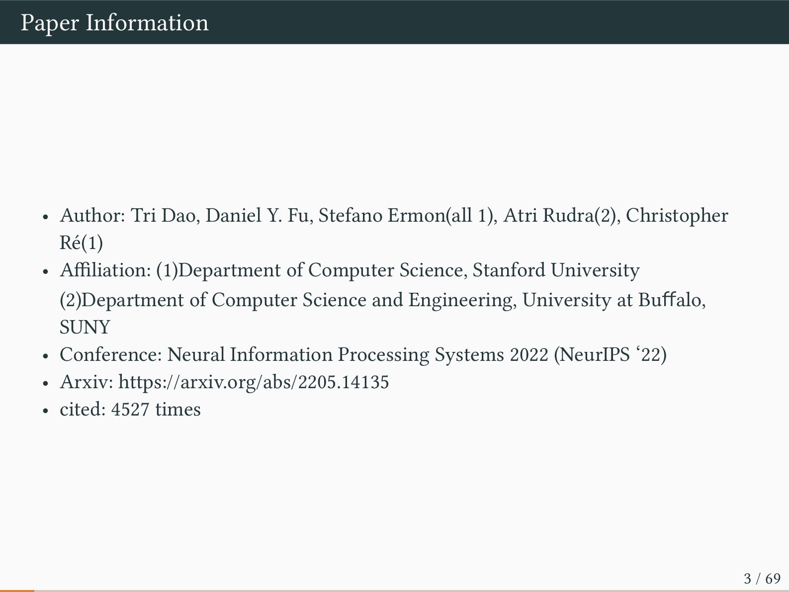
Ermon(all 1), Atri Rudra(2), Christopher Ré(1) • Affiliation: (1)Department of Computer Science, Stanford University (2)Department of Computer Science and Engineering, University at Buffalo, SUNY • Conference: Neural Information Processing Systems 2022 (NeurIPS ‘22) • Arxiv: https://arxiv.org/abs/2205.14135 • cited: 4527 times 3 / 69
LLM for architectures with cache hierarchies is memory I/O. This paper propose FlashAttention, an IO-aware exact attention algorithm that uses tiling to reduce the number of memory reads/writes between GPU high bandwidth memory (HBM) and GPU on-chip SRAM. 5 / 69
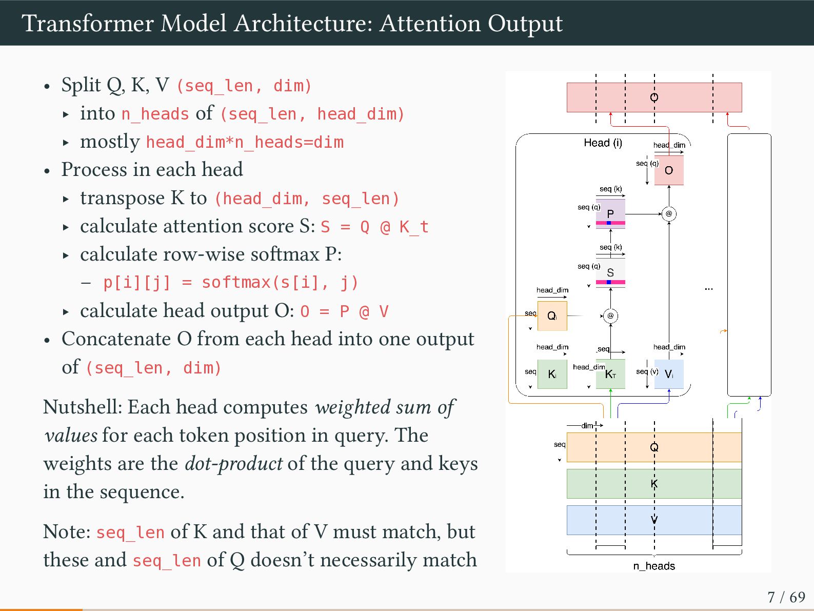
(seq_len, dim) ‣ into n_heads of (seq_len, head_dim) ‣ mostly head_dim*n_heads=dim • Process in each head ‣ transpose K to (head_dim, seq_len) ‣ calculate attention score S: S = Q @ K_t ‣ calculate row-wise softmax P: – p[i][j] = softmax(s[i], j) ‣ calculate head output O: O = P @ V • Concatenate O from each head into one output of (seq_len, dim) Nutshell: Each head computes weighted sum of values for each token position in query. The weights are the dot-product of the query and keys in the sequence. Note: seq_len of K and that of V must match, but these and seq_len of Q doesn’t necessarily match 7 / 69
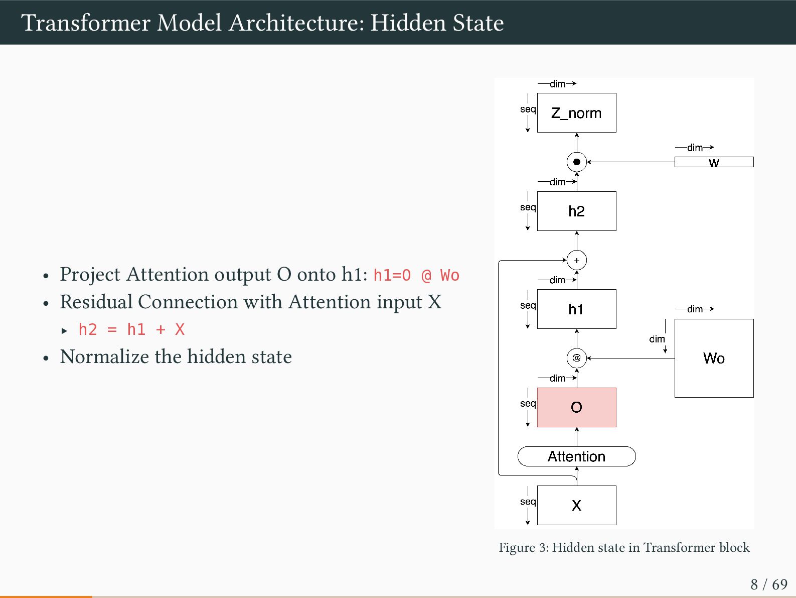
onto h1: h1=O @ Wo • Residual Connection with Attention input X ‣ h2 = h1 + X • Normalize the hidden state Figure 3: Hidden state in Transformer block 8 / 69
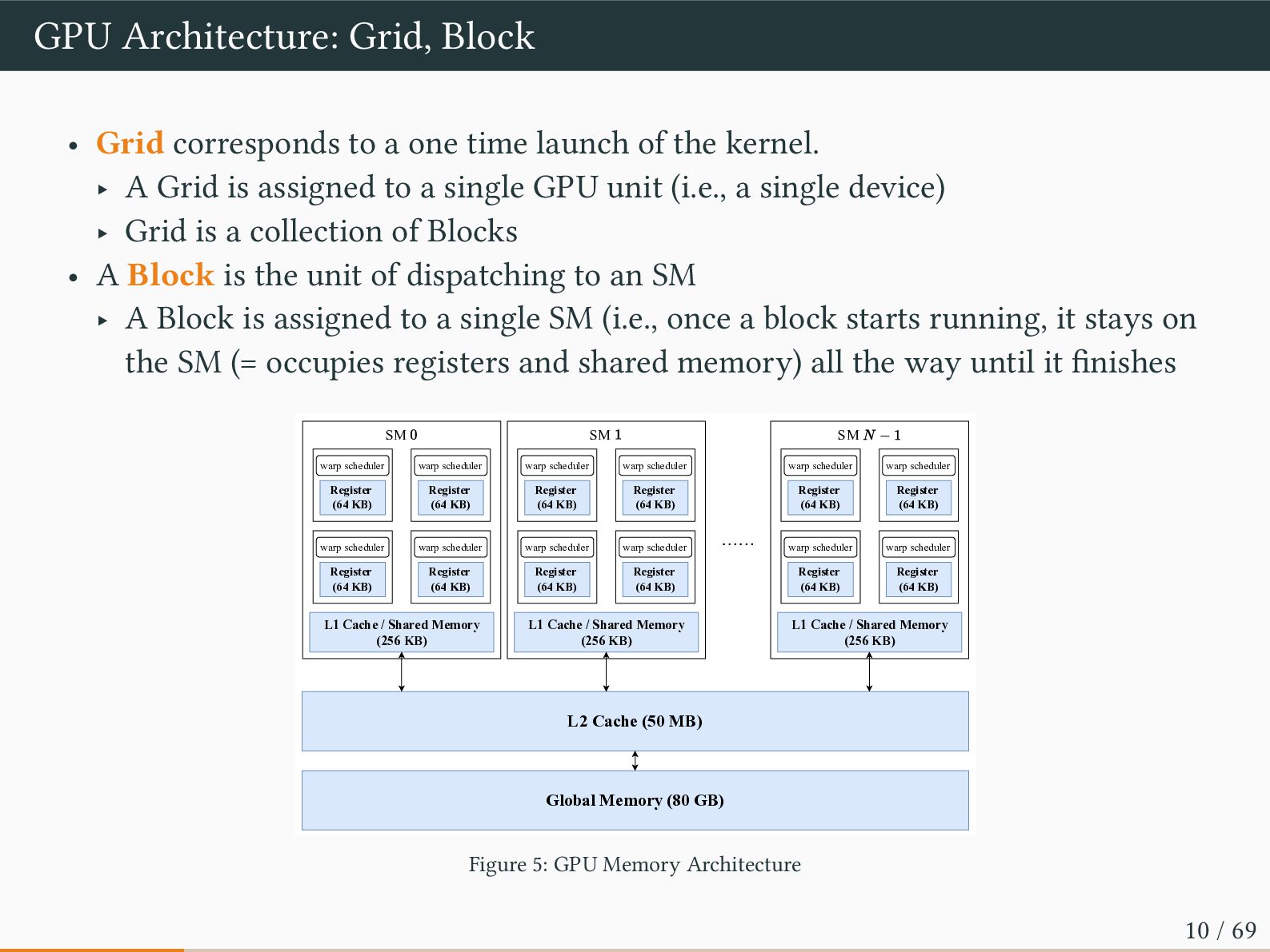
time launch of the kernel. ‣ A Grid is assigned to a single GPU unit (i.e., a single device) ‣ Grid is a collection of Blocks • A Block is the unit of dispatching to an SM ‣ A Block is assigned to a single SM (i.e., once a block starts running, it stays on the SM (= occupies registers and shared memory) all the way until it finishes L1 Cache / Shared Memory (256 KB) SM Register (64 KB) warp scheduler Register (64 KB) warp scheduler warp scheduler warp scheduler …… L2 Cache (50 MB) Global Memory (80 GB) Register (64 KB) Register (64 KB) L1 Cache / Shared Memory (256 KB) SM Register (64 KB) warp scheduler Register (64 KB) warp scheduler warp scheduler warp scheduler Register (64 KB) Register (64 KB) L1 Cache / Shared Memory (256 KB) SM Register (64 KB) warp scheduler Register (64 KB) warp scheduler warp scheduler warp scheduler Register (64 KB) Register (64 KB) Figure 5: GPU Memory Architecture 10 / 69
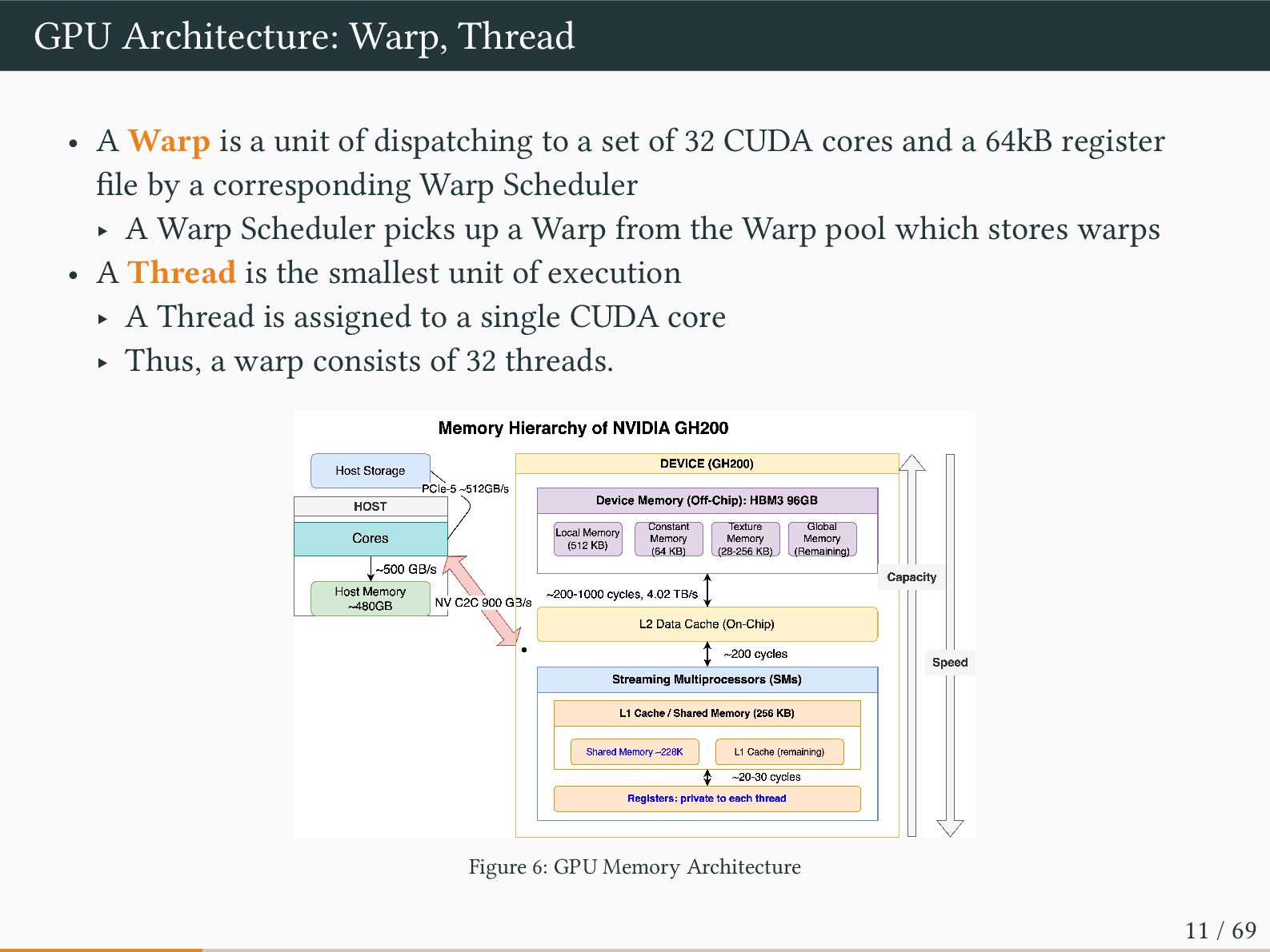
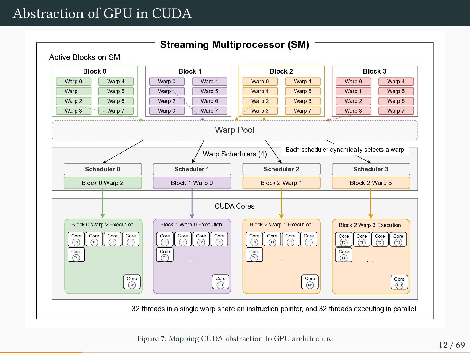
of dispatching to a set of 32 CUDA cores and a 64kB register file by a corresponding Warp Scheduler ‣ A Warp Scheduler picks up a Warp from the Warp pool which stores warps • A Thread is the smallest unit of execution ‣ A Thread is assigned to a single CUDA core ‣ Thus, a warp consists of 32 threads. Figure 6: GPU Memory Architecture 11 / 69
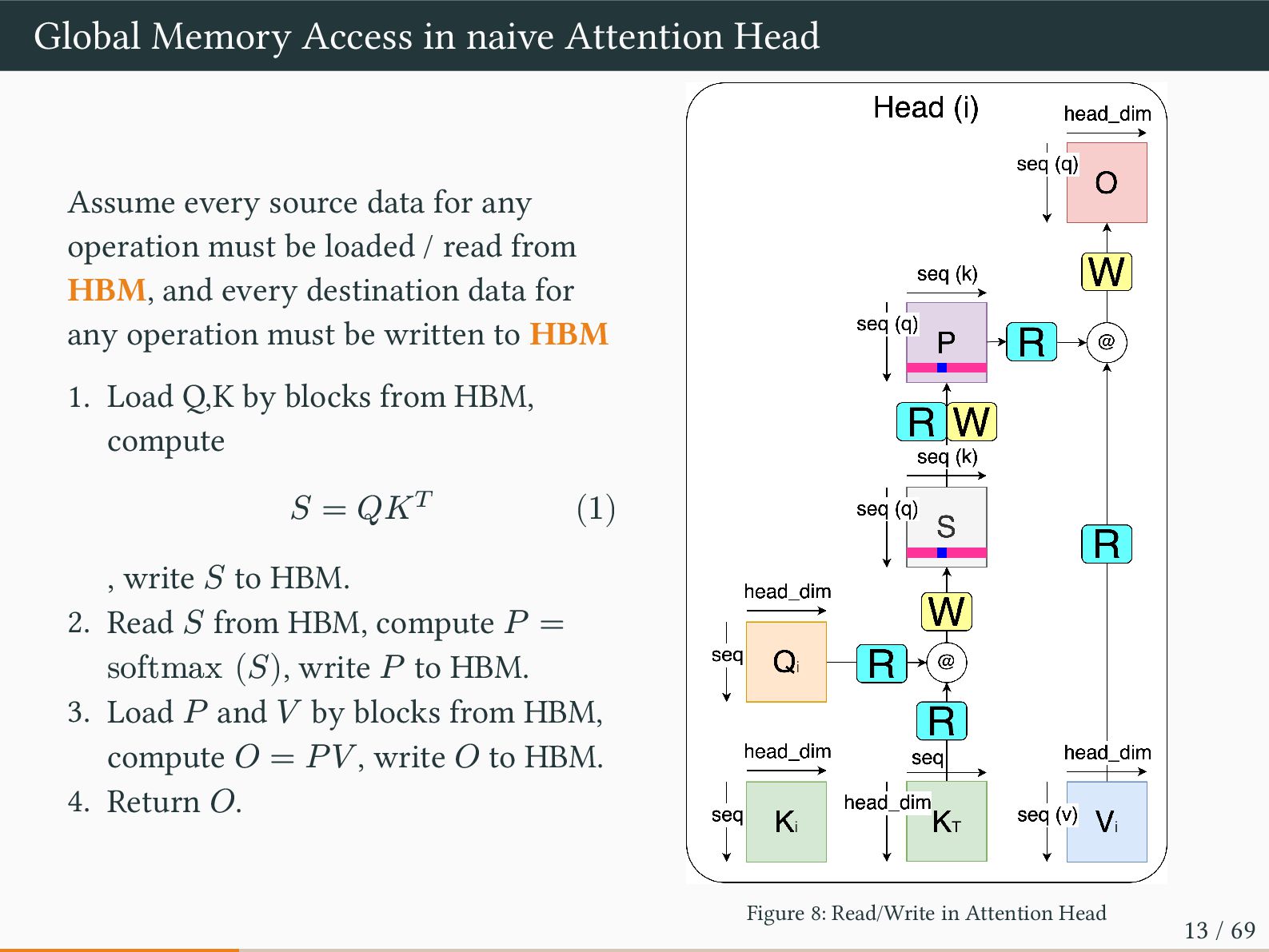
data for any operation must be loaded / read from HBM, and every destination data for any operation must be written to HBM 1. Load Q,K by blocks from HBM, compute 𝑆 = 𝑄𝐾𝑇 (1) , write 𝑆 to HBM. 2. Read 𝑆 from HBM, compute 𝑃 = softmax (𝑆), write 𝑃 to HBM. 3. Load 𝑃 and 𝑉 by blocks from HBM, compute 𝑂 = 𝑃𝑉 , write 𝑂 to HBM. 4. Return 𝑂. Figure 8: Read/Write in Attention Head 13 / 69
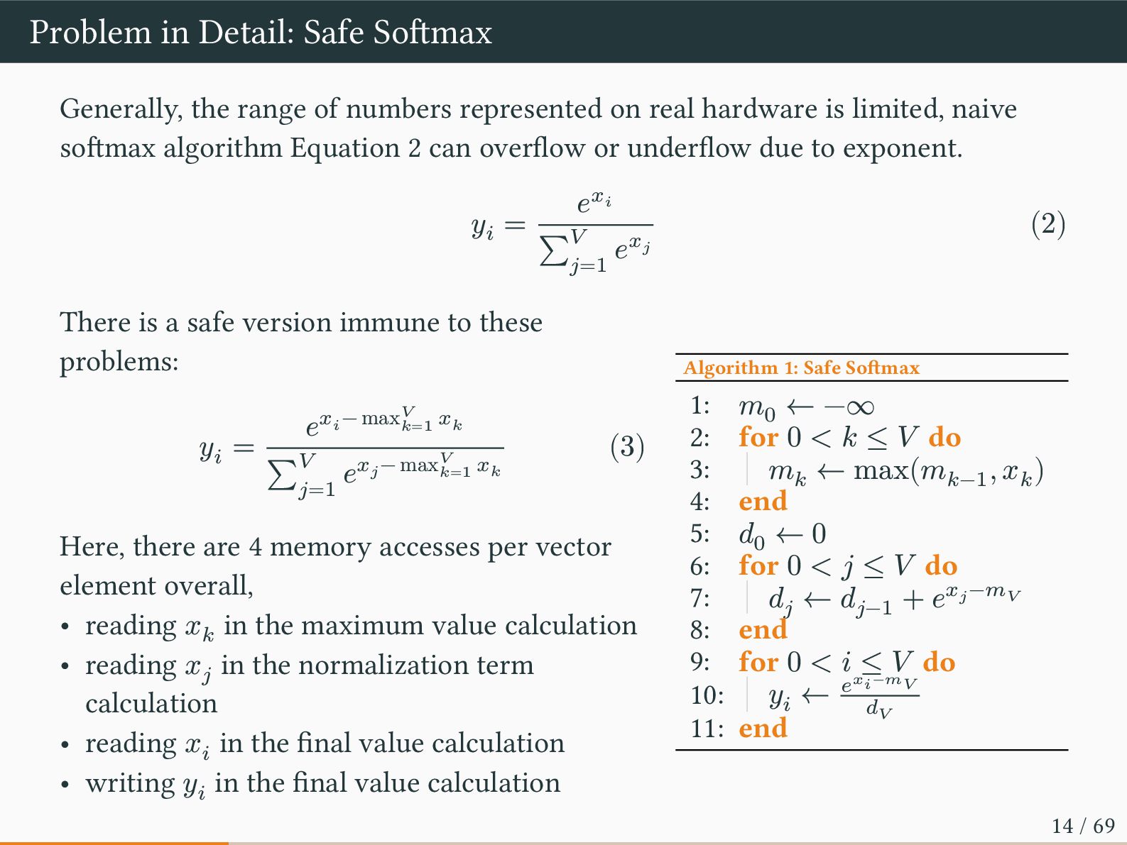
represented on real hardware is limited, naive softmax algorithm Equation 2 can overflow or underflow due to exponent. 𝑦𝑖 = 𝑒𝑥𝑖 ∑𝑉 𝑗=1 𝑒𝑥𝑗 (2) There is a safe version immune to these problems: 𝑦𝑖 = 𝑒𝑥𝑖 − max𝑉 𝑘=1 𝑥𝑘 ∑𝑉 𝑗=1 𝑒𝑥𝑗 − max𝑉 𝑘=1 𝑥𝑘 (3) Here, there are 4 memory accesses per vector element overall, • reading 𝑥𝑘 in the maximum value calculation • reading 𝑥𝑗 in the normalization term calculation • reading 𝑥𝑖 in the final value calculation • writing 𝑦𝑖 in the final value calculation Algorithm 1: Safe Softmax 1: 𝑚0 ← −∞ 2: for 0 < 𝑘 ≤ 𝑉 do 3: 𝑚𝑘 ← max(𝑚𝑘−1 , 𝑥𝑘 ) 4: end 5: 𝑑0 ← 0 6: for 0 < 𝑗 ≤ 𝑉 do 7: 𝑑𝑗 ← 𝑑𝑗−1 + 𝑒𝑥𝑗 −𝑚𝑉 8: end 9: for 0 < 𝑖 ≤ 𝑉 do 10: 𝑦𝑖 ← 𝑒𝑥𝑖−𝑚𝑉 𝑑𝑉 11: end 14 / 69
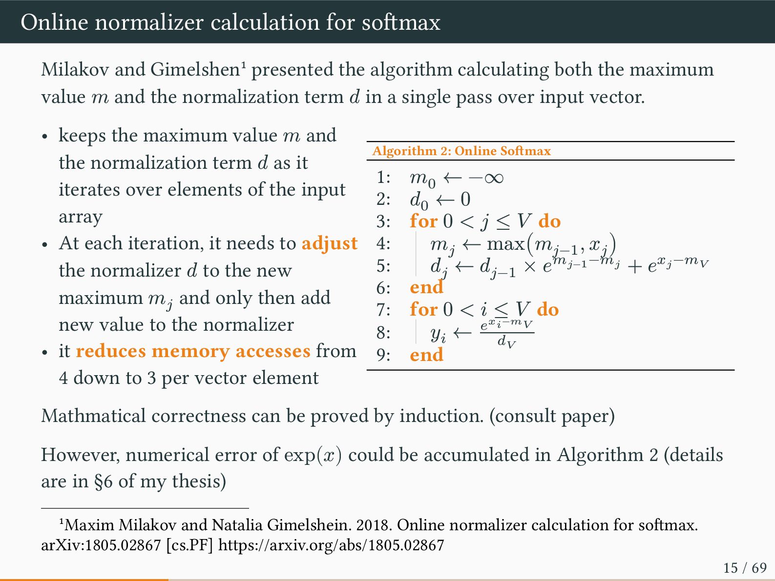
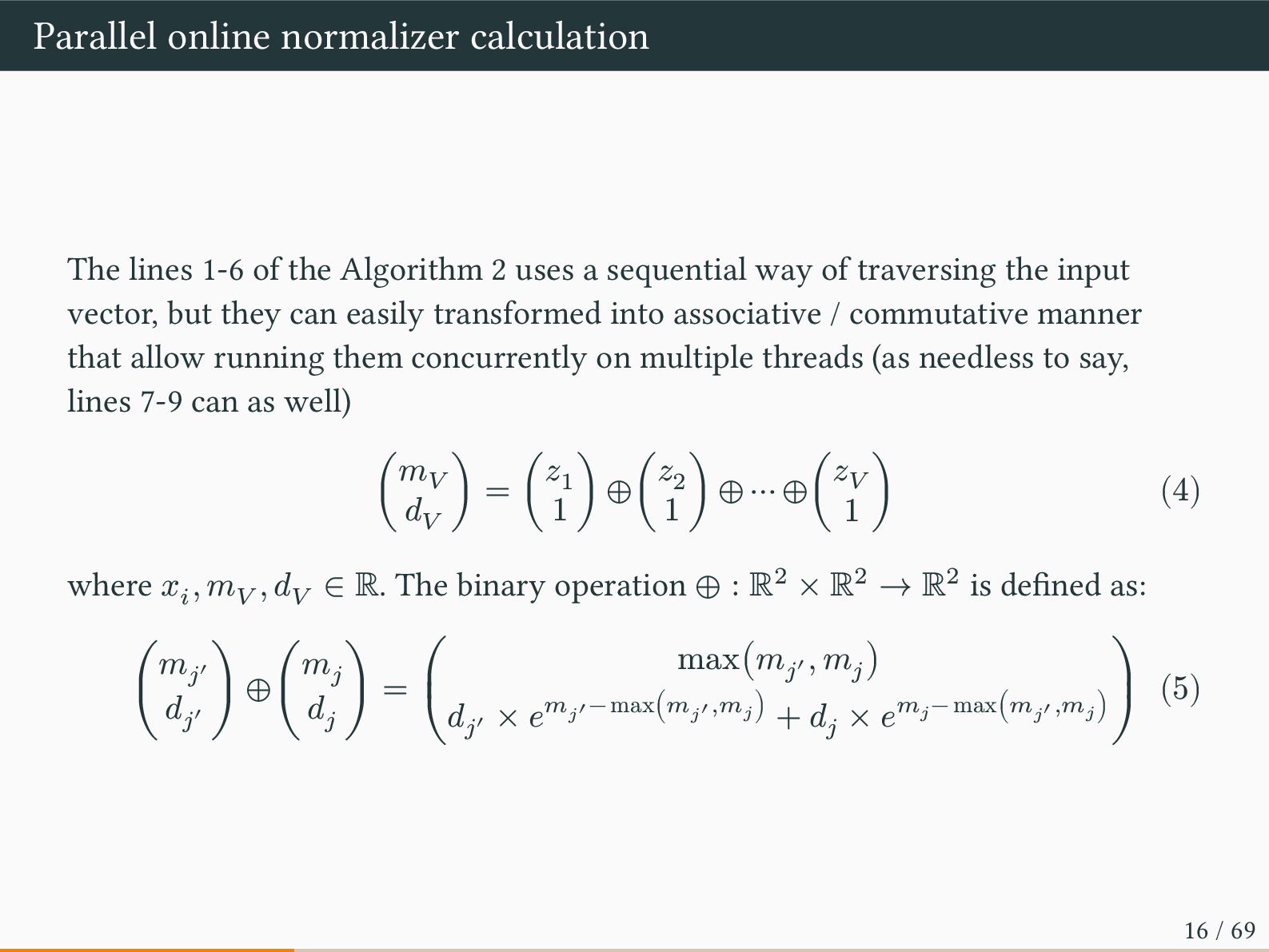
algorithm calculating both the maximum value 𝑚 and the normalization term 𝑑 in a single pass over input vector. • keeps the maximum value 𝑚 and the normalization term 𝑑 as it iterates over elements of the input array • At each iteration, it needs to adjust the normalizer 𝑑 to the new maximum 𝑚𝑗 and only then add new value to the normalizer • it reduces memory accesses from 4 down to 3 per vector element Algorithm 2: Online Softmax 1: 𝑚0 ← −∞ 2: 𝑑0 ← 0 3: for 0 < 𝑗 ≤ 𝑉 do 4: 𝑚𝑗 ← max(𝑚𝑗−1 , 𝑥𝑗 ) 5: 𝑑𝑗 ← 𝑑𝑗−1 × 𝑒𝑚𝑗−1 −𝑚𝑗 + 𝑒𝑥𝑗 −𝑚𝑉 6: end 7: for 0 < 𝑖 ≤ 𝑉 do 8: 𝑦𝑖 ← 𝑒𝑥𝑖−𝑚𝑉 𝑑𝑉 9: end Mathmatical correctness can be proved by induction. (consult paper) However, numerical error of exp(𝑥) could be accumulated in Algorithm 2 (details are in §6 of my thesis) 1Maxim Milakov and Natalia Gimelshein. 2018. Online normalizer calculation for softmax. arXiv:1805.02867 [cs.PF] https://arxiv.org/abs/1805.02867 15 / 69
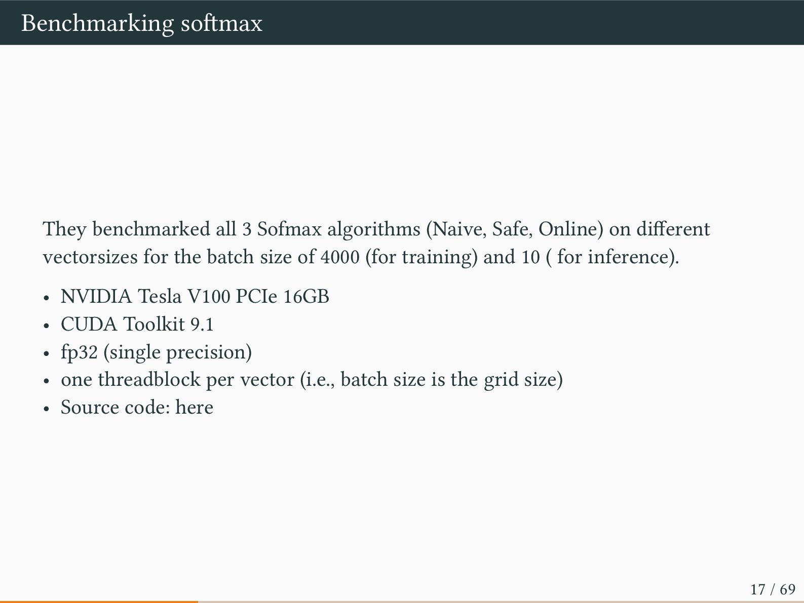
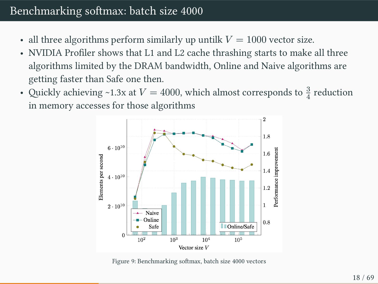
Online) on different vectorsizes for the batch size of 4000 (for training) and 10 ( for inference). • NVIDIA Tesla V100 PCIe 16GB • CUDA Toolkit 9.1 • fp32 (single precision) • one threadblock per vector (i.e., batch size is the grid size) • Source code: here 17 / 69
similarly up untilk 𝑉 = 1000 vector size. • NVIDIA Profiler shows that L1 and L2 cache thrashing starts to make all three algorithms limited by the DRAM bandwidth, Online and Naive algorithms are getting faster than Safe one then. • Quickly achieving ~1.3x at 𝑉 = 4000, which almost corresponds to 3 4 reduction in memory accesses for those algorithms Figure 9: Benchmarking softmax, batch size 4000 vectors 18 / 69
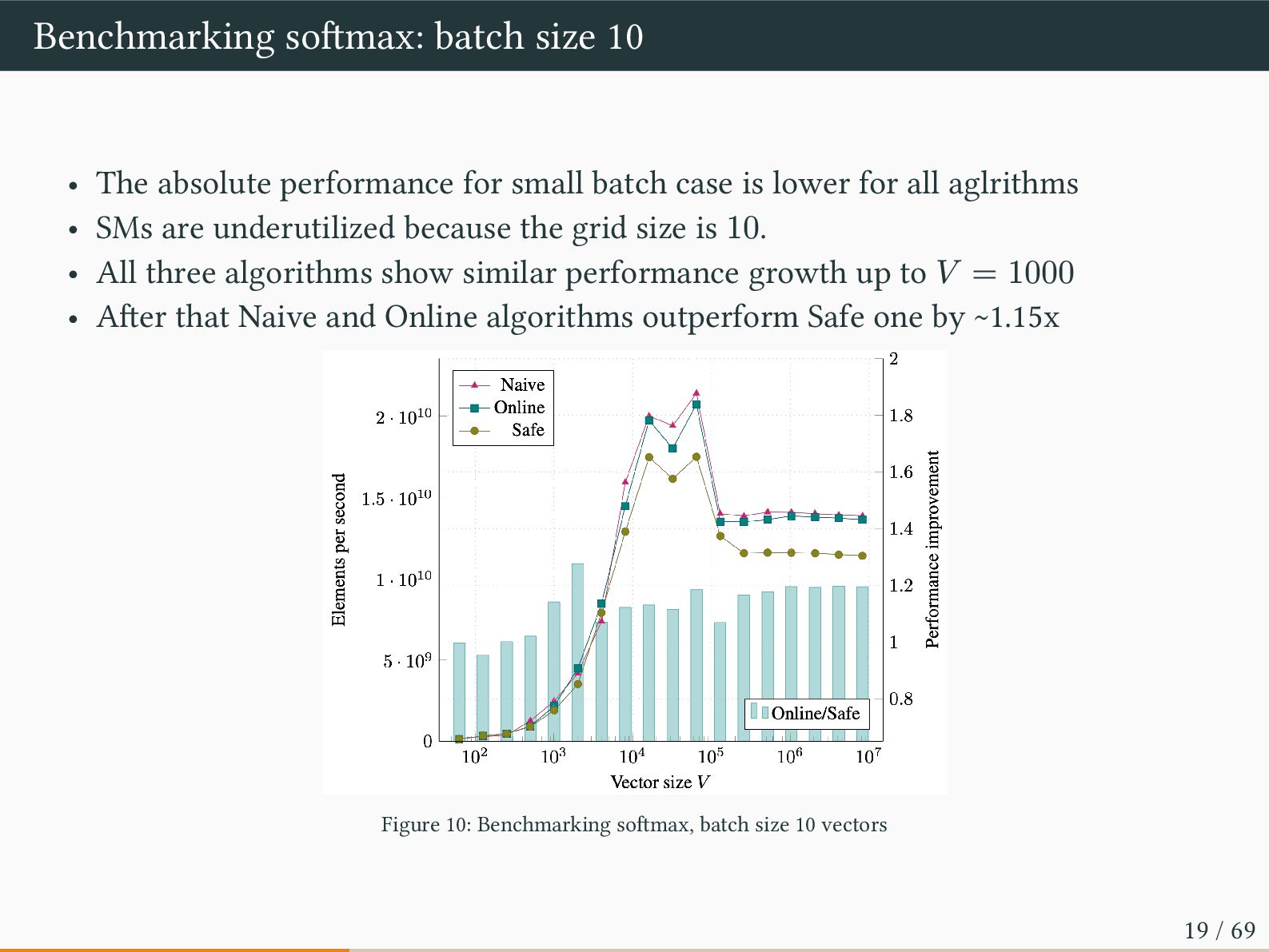
small batch case is lower for all aglrithms • SMs are underutilized because the grid size is 10. • All three algorithms show similar performance growth up to 𝑉 = 1000 • After that Naive and Online algorithms outperform Safe one by ~1.15x Figure 10: Benchmarking softmax, batch size 10 vectors 19 / 69
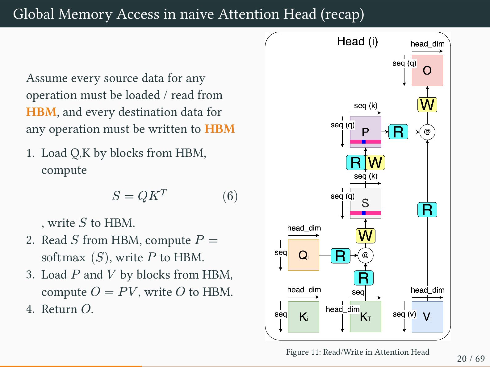
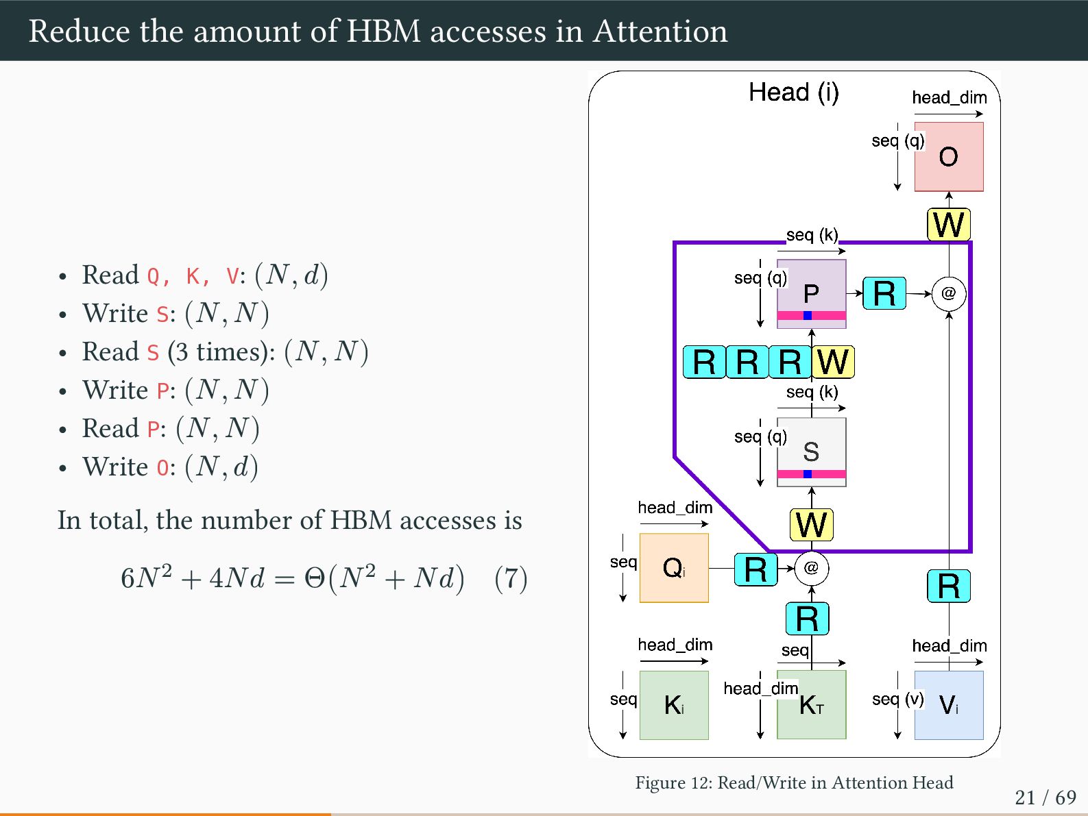
source data for any operation must be loaded / read from HBM, and every destination data for any operation must be written to HBM 1. Load Q,K by blocks from HBM, compute 𝑆 = 𝑄𝐾𝑇 (6) , write 𝑆 to HBM. 2. Read 𝑆 from HBM, compute 𝑃 = softmax (𝑆), write 𝑃 to HBM. 3. Load 𝑃 and 𝑉 by blocks from HBM, compute 𝑂 = 𝑃𝑉 , write 𝑂 to HBM. 4. Return 𝑂. Figure 11: Read/Write in Attention Head 20 / 69
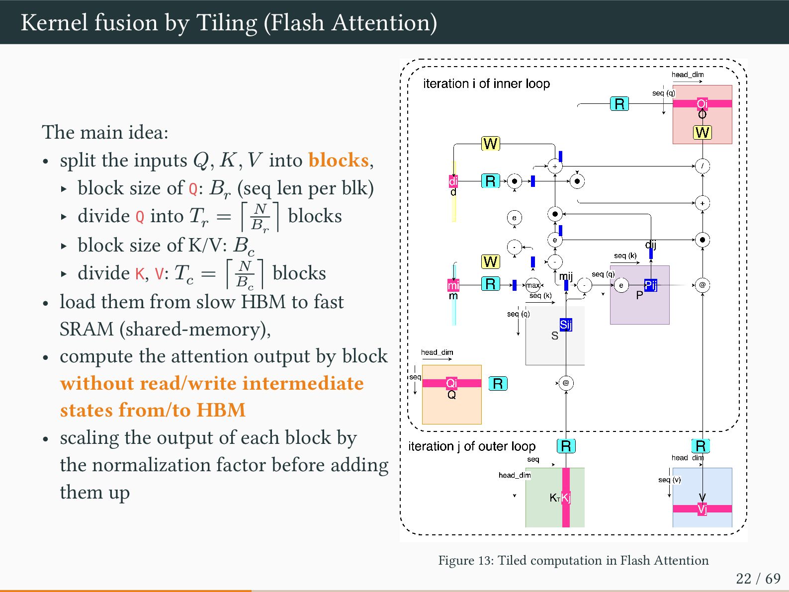
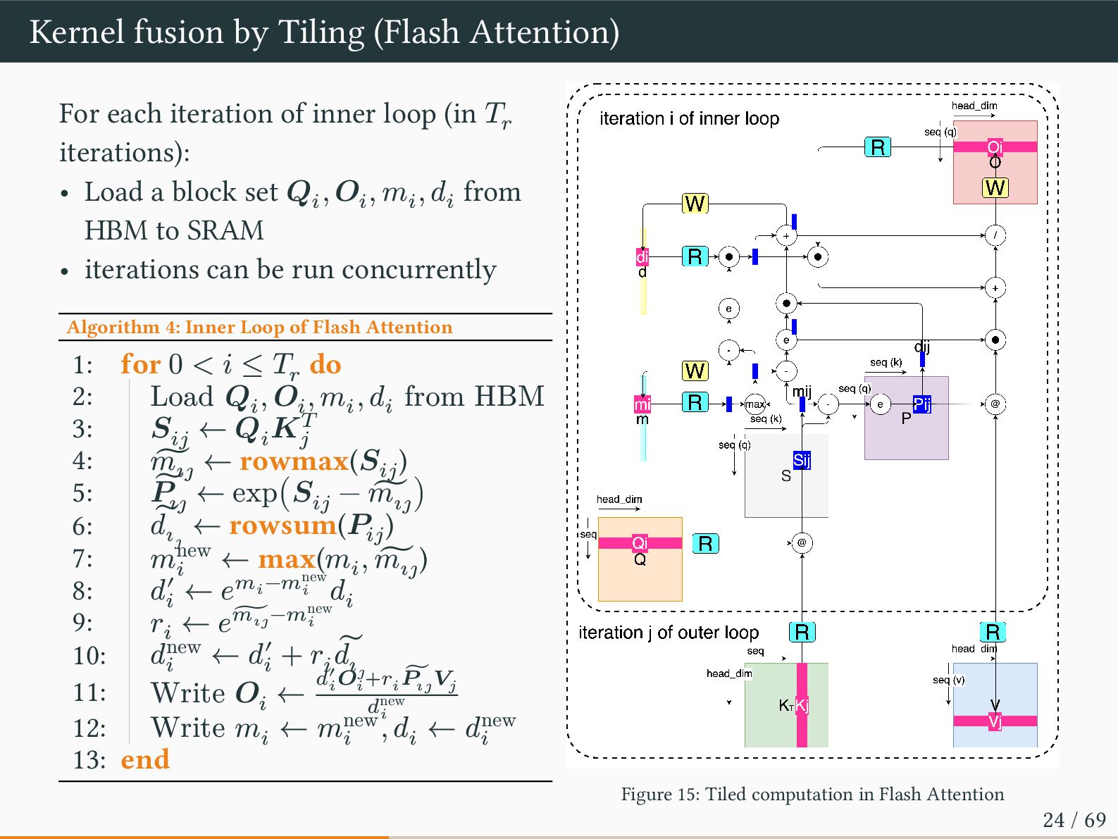
split the inputs 𝑄, 𝐾, 𝑉 into blocks, ‣ block size of Q: 𝐵𝑟 (seq len per blk) ‣ divide Q into 𝑇𝑟 = ⌈ 𝑁 𝐵𝑟 ⌉ blocks ‣ block size of K/V: 𝐵𝑐 ‣ divide K, V: 𝑇𝑐 = ⌈ 𝑁 𝐵𝑐 ⌉ blocks • load them from slow HBM to fast SRAM (shared-memory), • compute the attention output by block without read/write intermediate states from/to HBM • scaling the output of each block by the normalization factor before adding them up Figure 13: Tiled computation in Flash Attention 22 / 69
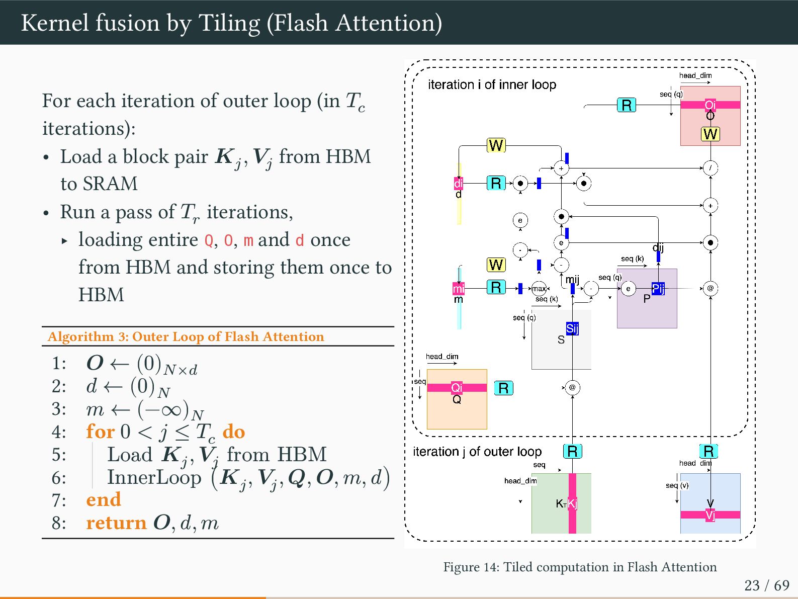
outer loop (in 𝑇𝑐 iterations): • Load a block pair 𝑲𝑗 , 𝑽𝑗 from HBM to SRAM • Run a pass of 𝑇𝑟 iterations, ‣ loading entire Q, O, m and d once from HBM and storing them once to HBM Algorithm 3: Outer Loop of Flash Attention 1: 𝑶 ← (0)𝑁×𝑑 2: 𝑑 ← (0)𝑁 3: 𝑚 ← (−∞)𝑁 4: for 0 < 𝑗 ≤ 𝑇𝑐 do 5: Load 𝑲𝑗 , 𝑽𝑗 from HBM 6: InnerLoop (𝑲𝑗 , 𝑽𝑗 , 𝑸, 𝑶, 𝑚, 𝑑) 7: end 8: return 𝑶, 𝑑, 𝑚 Figure 14: Tiled computation in Flash Attention 23 / 69
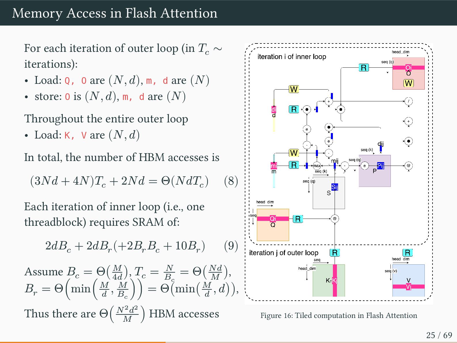
loop (in 𝑇𝑐 ∼ iterations): • Load: Q, O are (𝑁, 𝑑), m, d are (𝑁) • store: O is (𝑁, 𝑑), m, d are (𝑁) Throughout the entire outer loop • Load: K, V are (𝑁, 𝑑) In total, the number of HBM accesses is (3𝑁𝑑 + 4𝑁)𝑇𝑐 + 2𝑁𝑑 = Θ(𝑁𝑑𝑇𝑐 ) (8) Each iteration of inner loop (i.e., one threadblock) requires SRAM of: 2𝑑𝐵𝑐 + 2𝑑𝐵𝑟 (+2𝐵𝑟 𝐵𝑐 + 10𝐵𝑟 ) (9) Assume 𝐵𝑐 = Θ(𝑀 4𝑑 ), 𝑇𝑐 = 𝑁 𝐵𝑐 = Θ(𝑁𝑑 𝑀 ), 𝐵𝑟 = Θ(min(𝑀 𝑑 , 𝑀 𝐵𝑐 )) = Θ(min(𝑀 𝑑 , 𝑑)), Thus there are Θ(𝑁2𝑑2 𝑀 ) HBM accesses Figure 16: Tiled computation in Flash Attention 25 / 69
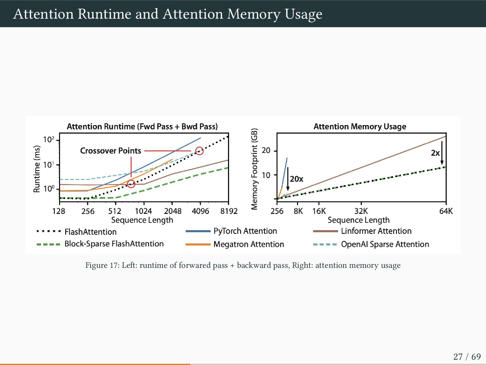
for BERT by 15%, and speeds up GPT-2 up to 3x over HuggingFace and 1.8x over Megatron-LM. • Speed enables quality: FlashAttention scales Transformers to longer sequence, yielding higher quality. FlashAttention trains GPT-2 with context length 4K faster than Megatron-LM which trains GPT-2 with context length 1K, which enables to achieve 0.7 better perplexity1 • Report attention runtime and memory benchmarks on single A100 GPU with 40GB HBM ‣ Runtime grows quadratically with sequence length, but FlashAttention runs significantly faster than exact attention baselines , up to 3x faster than the PyTorch implementation. ‣ FlashAttention still runs faster than many approximate/sparse attention mechanism (runtime is linearly growing) for short sequneces due to fewer memory accesses 1To what extent the model shows uncertainty in selecting the correct token Perplexity (𝑥1:𝑇 ) = exp(CrossEntropy (𝑥1:𝑇 )) = exp(− 1 𝑇 ∑ 𝑇 𝑡=1 log(𝑝(𝑥𝑡 |𝑥<𝑡 ))) (10) 26 / 69
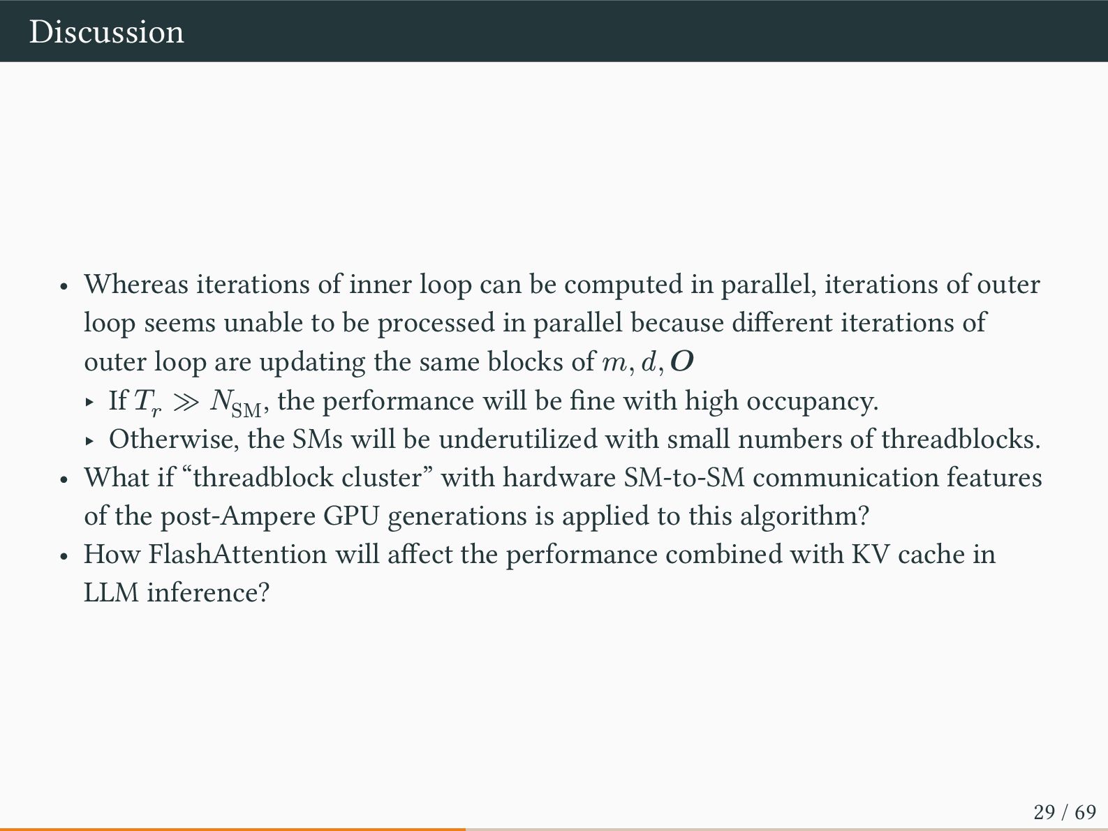
in parallel, iterations of outer loop seems unable to be processed in parallel because different iterations of outer loop are updating the same blocks of 𝑚, 𝑑, 𝑶 ‣ If 𝑇𝑟 ≫ 𝑁SM , the performance will be fine with high occupancy. ‣ Otherwise, the SMs will be underutilized with small numbers of threadblocks. • What if “threadblock cluster” with hardware SM-to-SM communication features of the post-Ampere GPU generations is applied to this algorithm? • How FlashAttention will affect the performance combined with KV cache in LLM inference? 29 / 69
Ziming Miao(2) Jilong Xue(2) Lingxiao Ma(2) Fan Yang(2) Luo Mai • Affiliation: (1)University of Edinburgh (2)Microsoft Research • Conference: Proceedings of the 19th USENIX Conference on Operating Systems Design and Implementation (OSDI ‘25) • Arxiv: https://arxiv.org/abs/2502.04563 • cited: 13 times 31 / 69
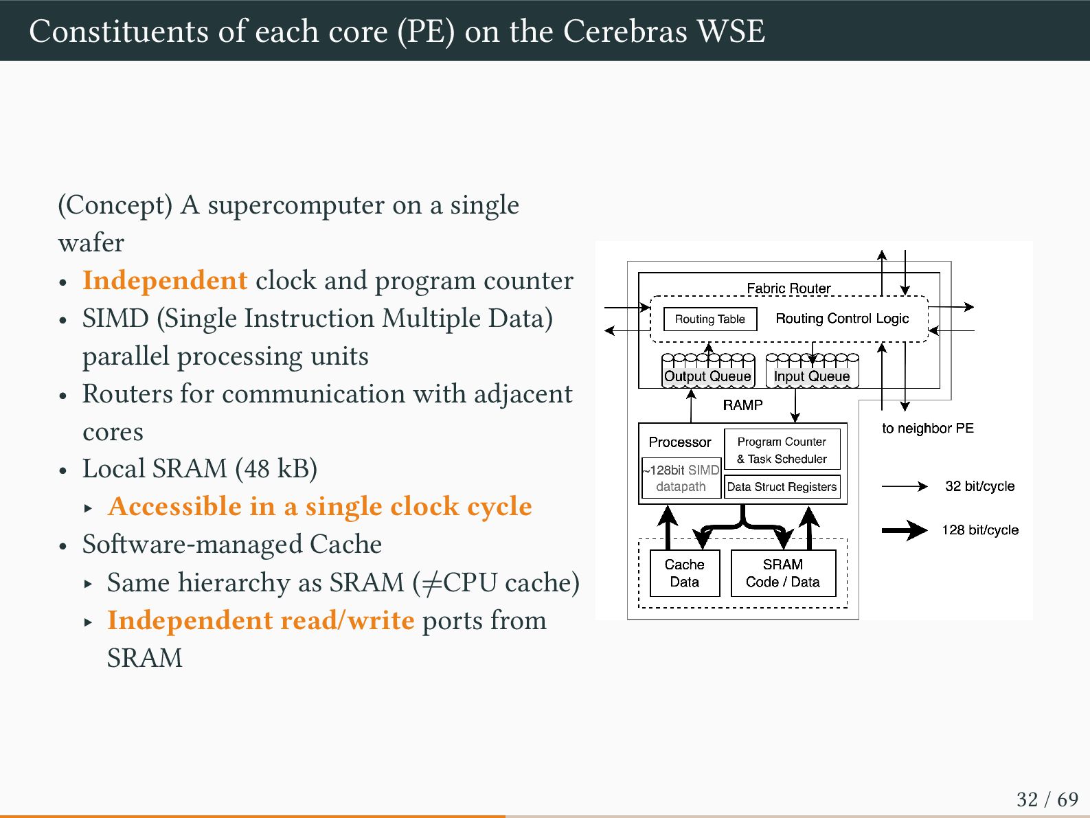
A supercomputer on a single wafer • Independent clock and program counter • SIMD (Single Instruction Multiple Data) parallel processing units • Routers for communication with adjacent cores • Local SRAM (48 kB) ‣ Accessible in a single clock cycle • Software-managed Cache ‣ Same hierarchy as SRAM (≠CPU cache) ‣ Independent read/write ports from SRAM 32 / 69
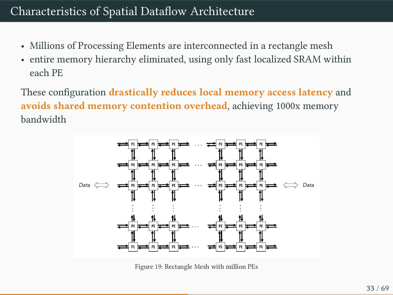
are interconnected in a rectangle mesh • entire memory hierarchy eliminated, using only fast localized SRAM within each PE These configuration drastically reduces local memory access latency and avoids shared memory contention overhead, achieving 1000x memory bandwidth Figure 19: Rectangle Mesh with million PEs 33 / 69
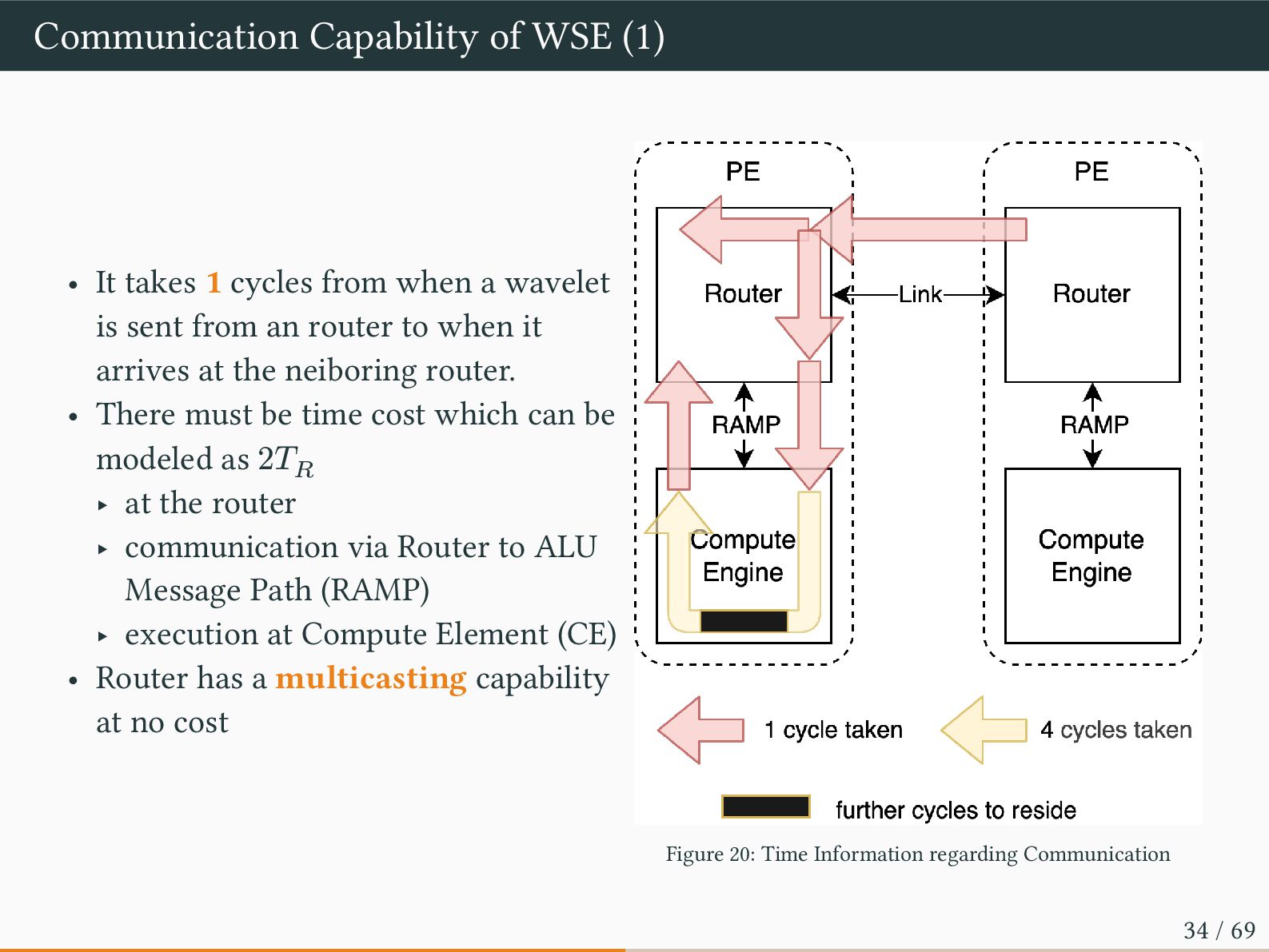
from when a wavelet is sent from an router to when it arrives at the neiboring router. • There must be time cost which can be modeled as 2𝑇𝑅 ‣ at the router ‣ communication via Router to ALU Message Path (RAMP) ‣ execution at Compute Element (CE) • Router has a multicasting capability at no cost Figure 20: Time Information regarding Communication 34 / 69
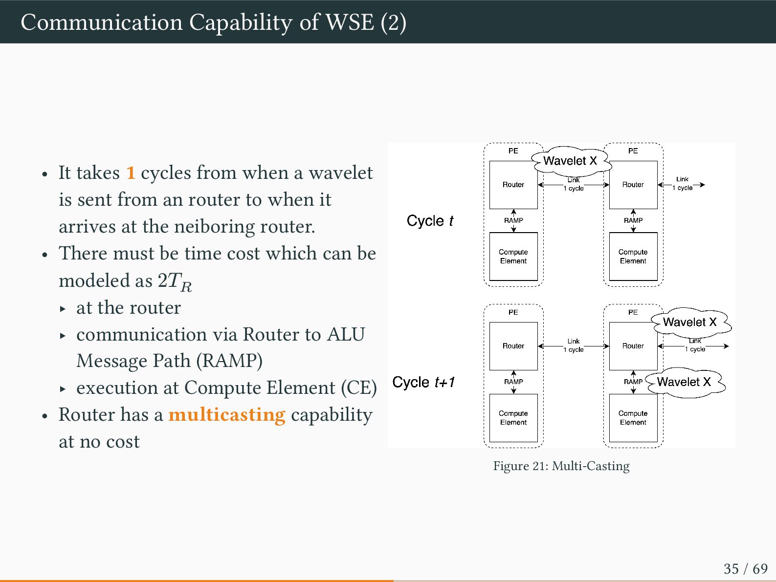
from when a wavelet is sent from an router to when it arrives at the neiboring router. • There must be time cost which can be modeled as 2𝑇𝑅 ‣ at the router ‣ communication via Router to ALU Message Path (RAMP) ‣ execution at Compute Element (CE) • Router has a multicasting capability at no cost Figure 21: Multi-Casting 35 / 69
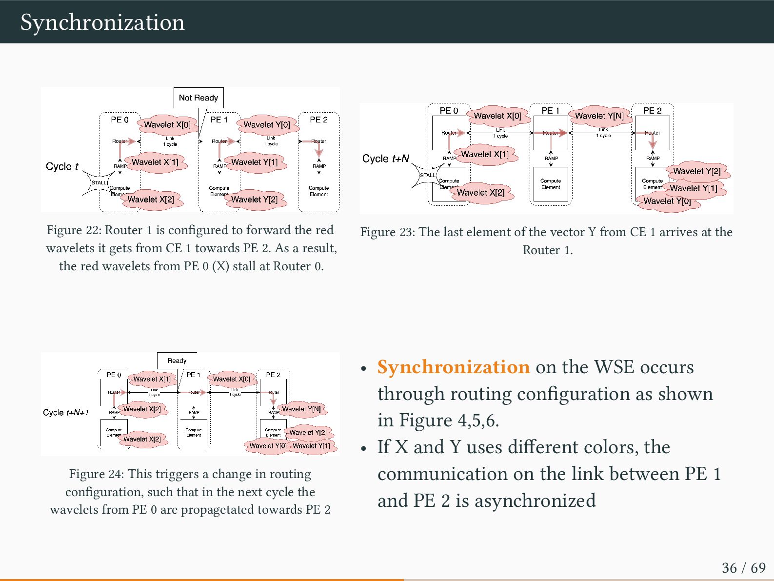
red wavelets it gets from CE 1 towards PE 2. As a result, the red wavelets from PE 0 (X) stall at Router 0. Figure 23: The last element of the vector Y from CE 1 arrives at the Router 1. Figure 24: This triggers a change in routing configuration, such that in the next cycle the wavelets from PE 0 are propagetated towards PE 2 • Synchronization on the WSE occurs through routing configuration as shown in Figure 4,5,6. • If X and Y uses different colors, the communication on the link between PE 1 and PE 2 is asynchronized 36 / 69
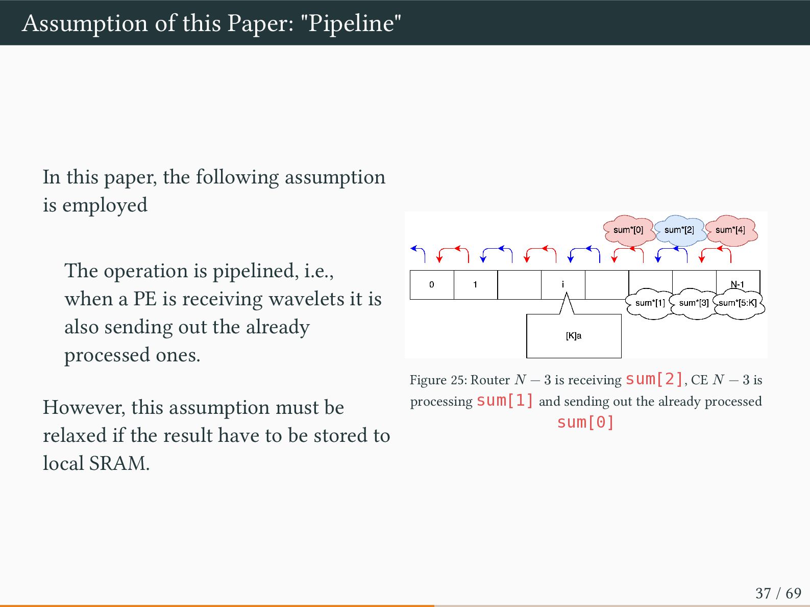
assumption is employed The operation is pipelined, i.e., when a PE is receiving wavelets it is also sending out the already processed ones. However, this assumption must be relaxed if the result have to be stored to local SRAM. Figure 25: Router 𝑁 − 3 is receiving sum[2], CE 𝑁 − 3 is processing sum[1] and sending out the already processed sum[0] 37 / 69
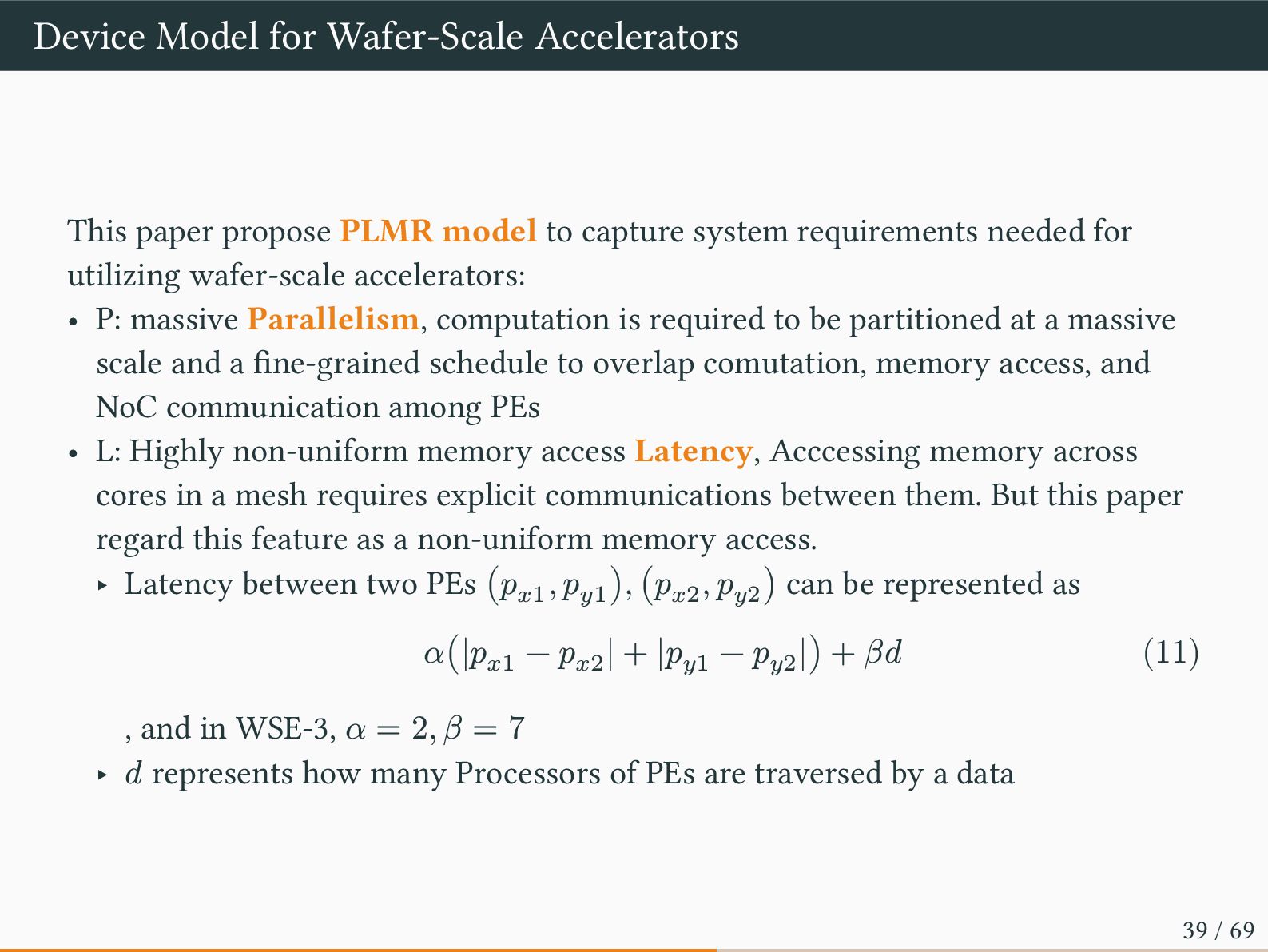
to capture system requirements needed for utilizing wafer-scale accelerators: • P: massive Parallelism, computation is required to be partitioned at a massive scale and a fine-grained schedule to overlap comutation, memory access, and NoC communication among PEs • L: Highly non-uniform memory access Latency, Acccessing memory across cores in a mesh requires explicit communications between them. But this paper regard this feature as a non-uniform memory access. ‣ Latency between two PEs (𝑝𝑥1 , 𝑝𝑦1 ), (𝑝𝑥2 , 𝑝𝑦2 ) can be represented as 𝛼(|𝑝𝑥1 − 𝑝𝑥2 | + |𝑝𝑦1 − 𝑝𝑦2 |) + 𝛽𝑑 (11) , and in WSE-3, 𝛼 = 2, 𝛽 = 7 ‣ 𝑑 represents how many Processors of PEs are traversed by a data 39 / 69
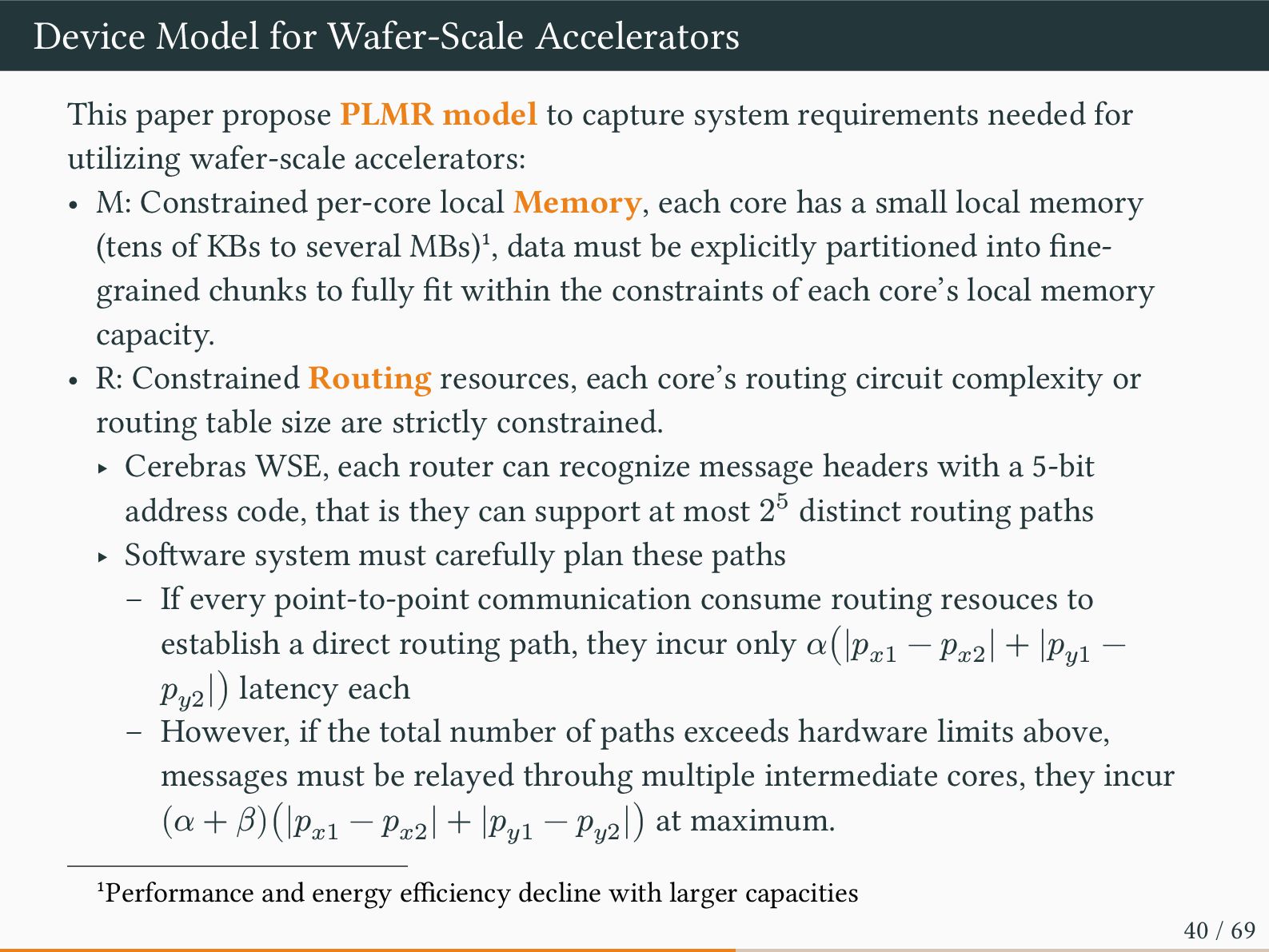
to capture system requirements needed for utilizing wafer-scale accelerators: • M: Constrained per-core local Memory, each core has a small local memory (tens of KBs to several MBs)1, data must be explicitly partitioned into fine- grained chunks to fully fit within the constraints of each core’s local memory capacity. • R: Constrained Routing resources, each core’s routing circuit complexity or routing table size are strictly constrained. ‣ Cerebras WSE, each router can recognize message headers with a 5-bit address code, that is they can support at most 25 distinct routing paths ‣ Software system must carefully plan these paths – If every point-to-point communication consume routing resouces to establish a direct routing path, they incur only 𝛼(|𝑝𝑥1 − 𝑝𝑥2 | + |𝑝𝑦1 − 𝑝𝑦2 |) latency each – However, if the total number of paths exceeds hardware limits above, messages must be relayed throuhg multiple intermediate cores, they incur (𝛼 + 𝛽)(|𝑝𝑥1 − 𝑝𝑥2 | + |𝑝𝑦1 − 𝑝𝑦2 |) at maximum. 1Performance and energy efficiency decline with larger capacities 40 / 69
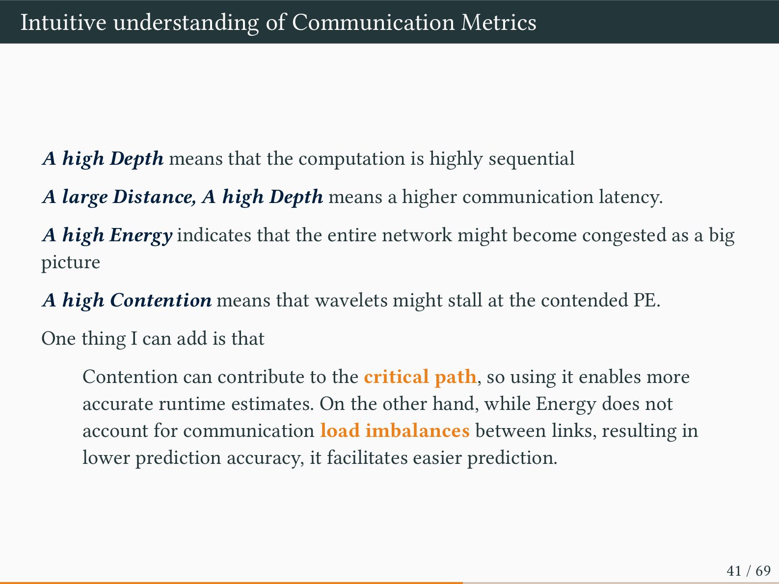
the computation is highly sequential A large Distance, A high Depth means a higher communication latency. A high Energy indicates that the entire network might become congested as a big picture A high Contention means that wavelets might stall at the contended PE. One thing I can add is that Contention can contribute to the critical path, so using it enables more accurate runtime estimates. On the other hand, while Energy does not account for communication load imbalances between links, resulting in lower prediction accuracy, it facilitates easier prediction. 41 / 69
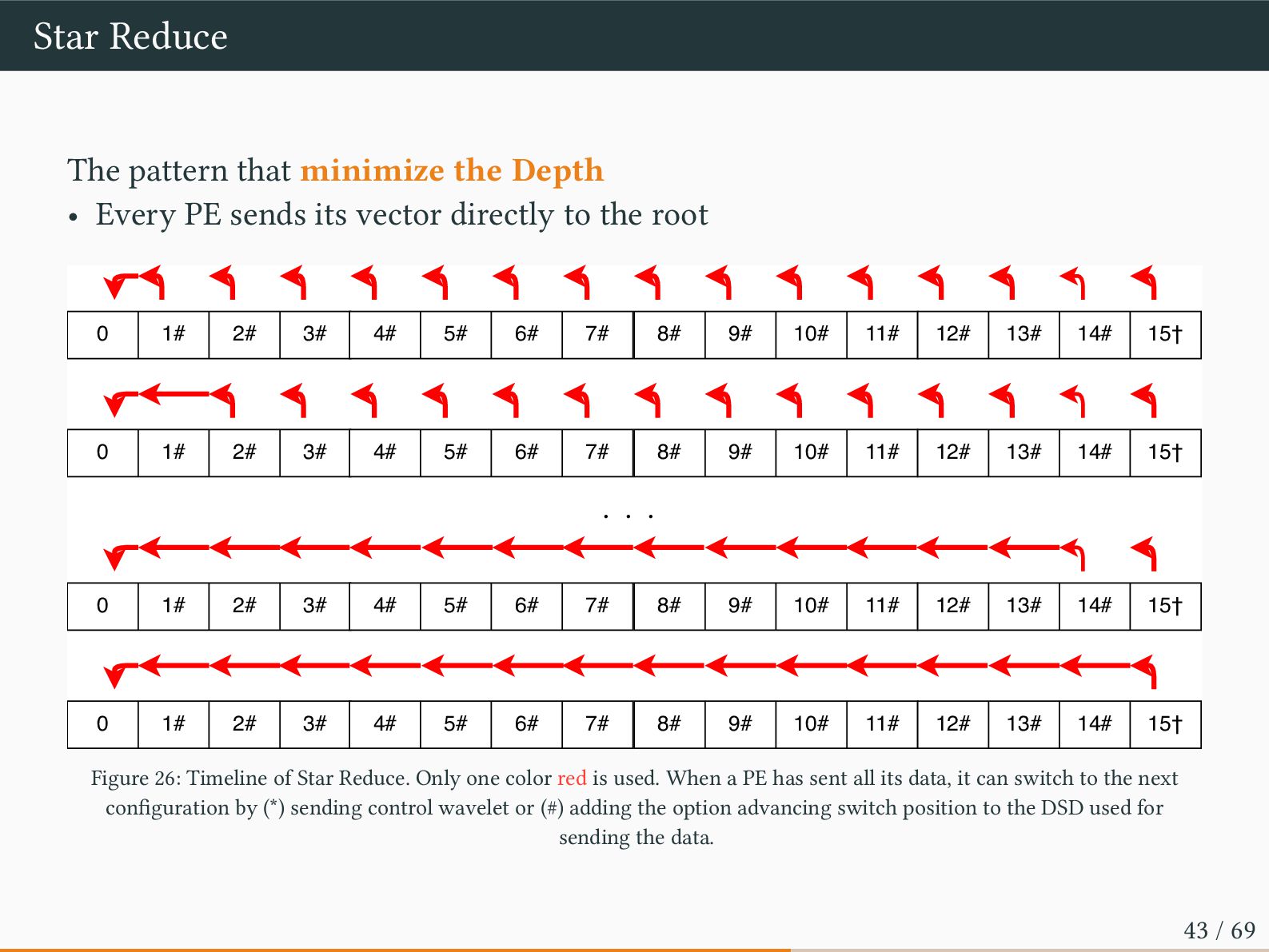
PE sends its vector directly to the root 0 1# 2# 3# 4# 5# 6# 7# 8# 9# 10# 11# 12# 13# 14# 15† 0 1# 2# 3# 4# 5# 6# 7# 8# 9# 10# 11# 12# 13# 14# 15† 0 1# 2# 3# 4# 5# 6# 7# 8# 9# 10# 11# 12# 13# 14# 15† 0 1# 2# 3# 4# 5# 6# 7# 8# 9# 10# 11# 12# 13# 14# 15† ・・・ Figure 26: Timeline of Star Reduce. Only one color red is used. When a PE has sent all its data, it can switch to the next configuration by (*) sending control wavelet or (#) adding the option advancing switch position to the DSD used for sending the data. 43 / 69
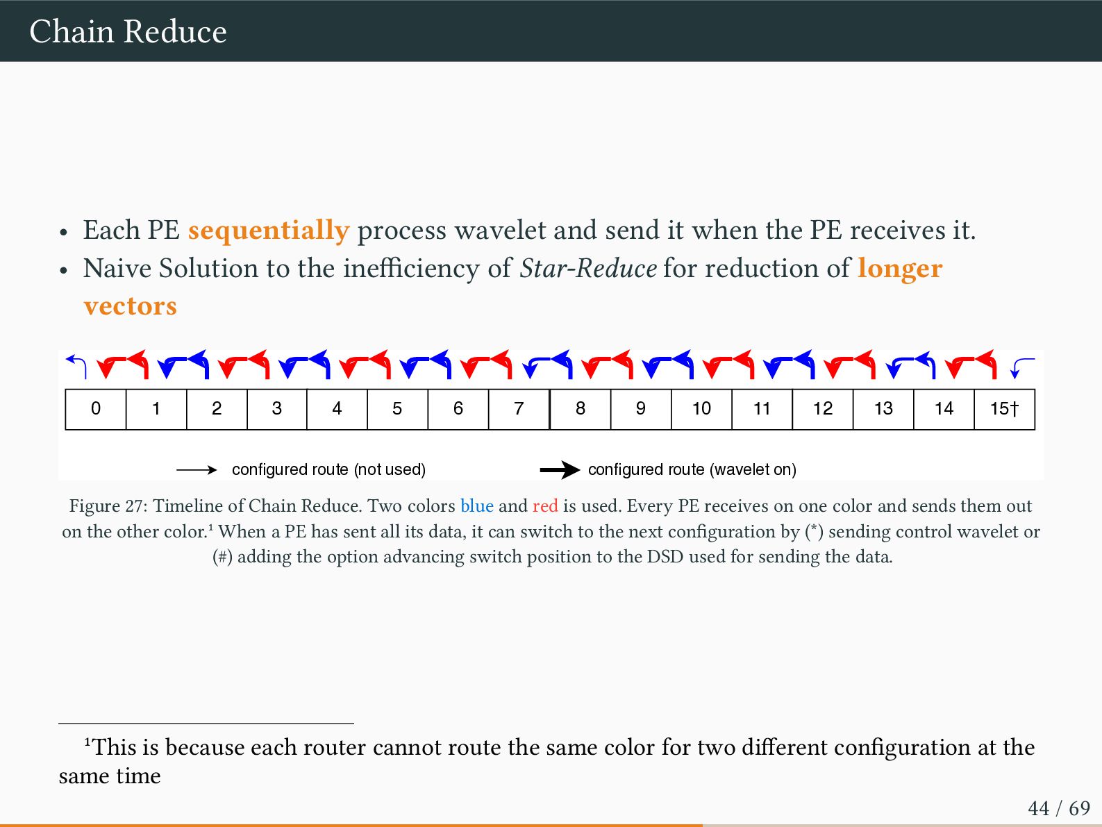
it when the PE receives it. • Naive Solution to the inefficiency of Star-Reduce for reduction of longer vectors configured route (not used) configured route (wavelet on) 0 1 2 3 4 5 6 7 8 9 10 11 12 13 14 15† Figure 27: Timeline of Chain Reduce. Two colors blue and red is used. Every PE receives on one color and sends them out on the other color.1 When a PE has sent all its data, it can switch to the next configuration by (*) sending control wavelet or (#) adding the option advancing switch position to the DSD used for sending the data. 1This is because each router cannot route the same color for two different configuration at the same time 44 / 69
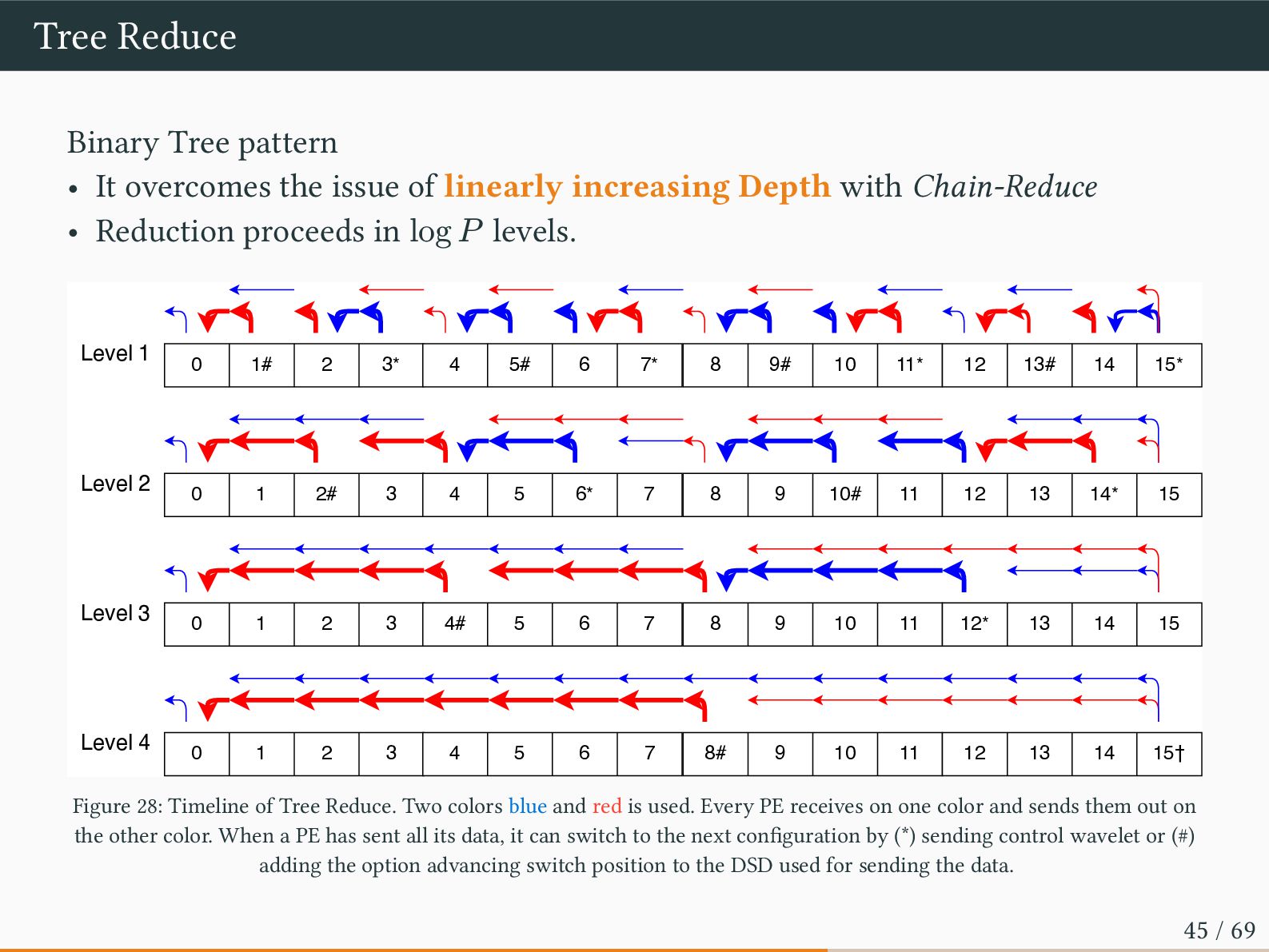
of linearly increasing Depth with Chain-Reduce • Reduction proceeds in log 𝑃 levels. Level 1 Level 2 Level 3 Level 4 0 1# 2 3* 4 5# 6 7* 8 9# 10 11* 12 13# 14 15* 0 1 2# 3 4 5 6* 7 8 9 10# 11 12 13 14* 15 0 1 2 3 4# 5 6 7 8 9 10 11 12* 13 14 15 0 1 2 3 4 5 6 7 8# 9 10 11 12 13 14 15† Figure 28: Timeline of Tree Reduce. Two colors blue and red is used. Every PE receives on one color and sends them out on the other color. When a PE has sent all its data, it can switch to the next configuration by (*) sending control wavelet or (#) adding the option advancing switch position to the DSD used for sending the data. 45 / 69
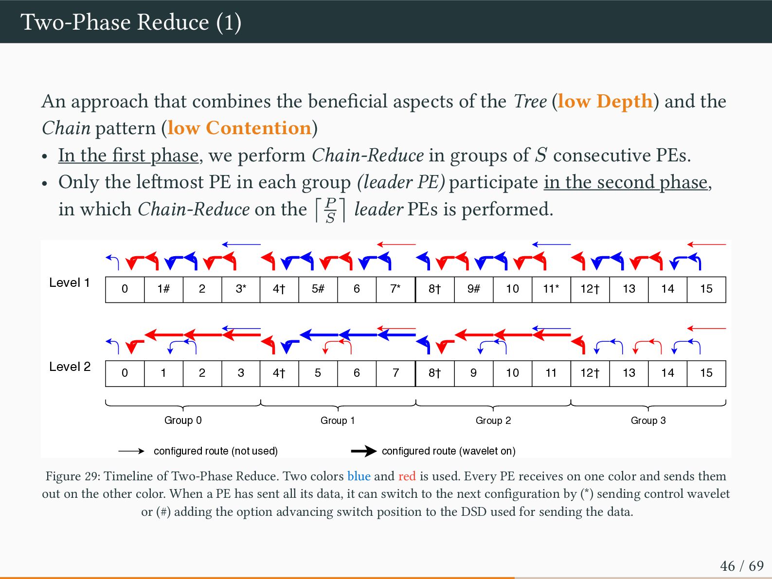
of the Tree (low Depth) and the Chain pattern (low Contention) • In the first phase, we perform Chain-Reduce in groups of 𝑆 consecutive PEs. • Only the leftmost PE in each group (leader PE) participate in the second phase, in which Chain-Reduce on the ⌈𝑃 𝑆 ⌉ leader PEs is performed. Level 1 Level 2 Group 0 Group 1 Group 2 Group 3 configured route (not used) configured route (wavelet on) 0 1# 2 3* 4† 5# 6 7* 8† 9# 10 11* 12† 13 14 15 0 1 2 3 4† 5 6 7 8† 9 10 11 12† 13 14 15 Figure 29: Timeline of Two-Phase Reduce. Two colors blue and red is used. Every PE receives on one color and sends them out on the other color. When a PE has sent all its data, it can switch to the next configuration by (*) sending control wavelet or (#) adding the option advancing switch position to the DSD used for sending the data. 46 / 69
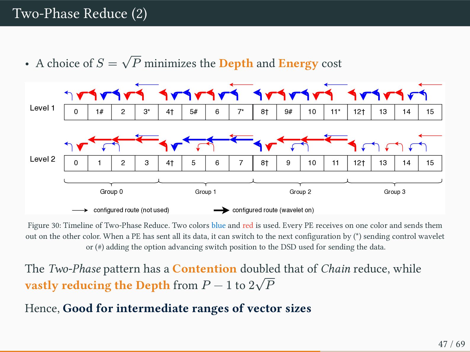
𝑃 minimizes the Depth and Energy cost Level 1 Level 2 Group 0 Group 1 Group 2 Group 3 configured route (not used) configured route (wavelet on) 0 1# 2 3* 4† 5# 6 7* 8† 9# 10 11* 12† 13 14 15 0 1 2 3 4† 5 6 7 8† 9 10 11 12† 13 14 15 Figure 30: Timeline of Two-Phase Reduce. Two colors blue and red is used. Every PE receives on one color and sends them out on the other color. When a PE has sent all its data, it can switch to the next configuration by (*) sending control wavelet or (#) adding the option advancing switch position to the DSD used for sending the data. The Two-Phase pattern has a Contention doubled that of Chain reduce, while vastly reducing the Depth from 𝑃 − 1 to 2 √ 𝑃 Hence, Good for intermediate ranges of vector sizes 47 / 69
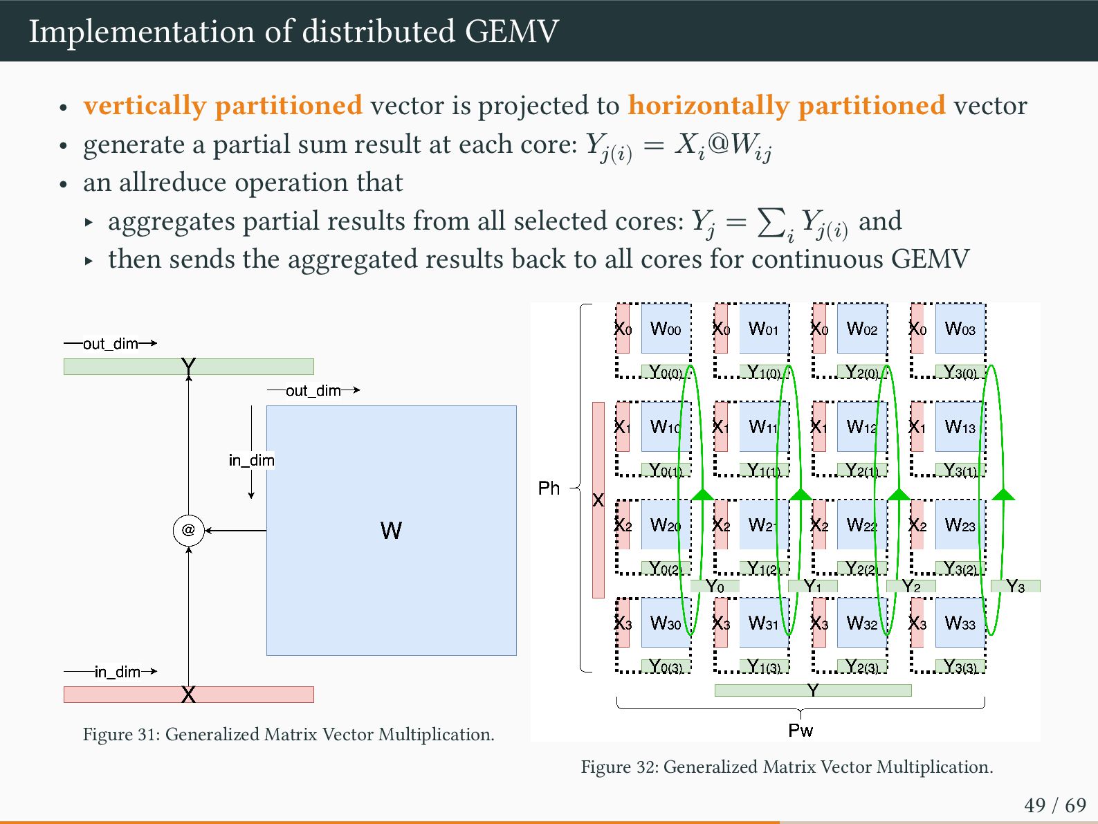
to horizontally partitioned vector • generate a partial sum result at each core: 𝑌𝑗(𝑖) = 𝑋𝑖 @𝑊𝑖𝑗 • an allreduce operation that ‣ aggregates partial results from all selected cores: 𝑌𝑗 = ∑ 𝑖 𝑌𝑗(𝑖) and ‣ then sends the aggregated results back to all cores for continuous GEMV Figure 31: Generalized Matrix Vector Multiplication. Figure 32: Generalized Matrix Vector Multiplication. 49 / 69
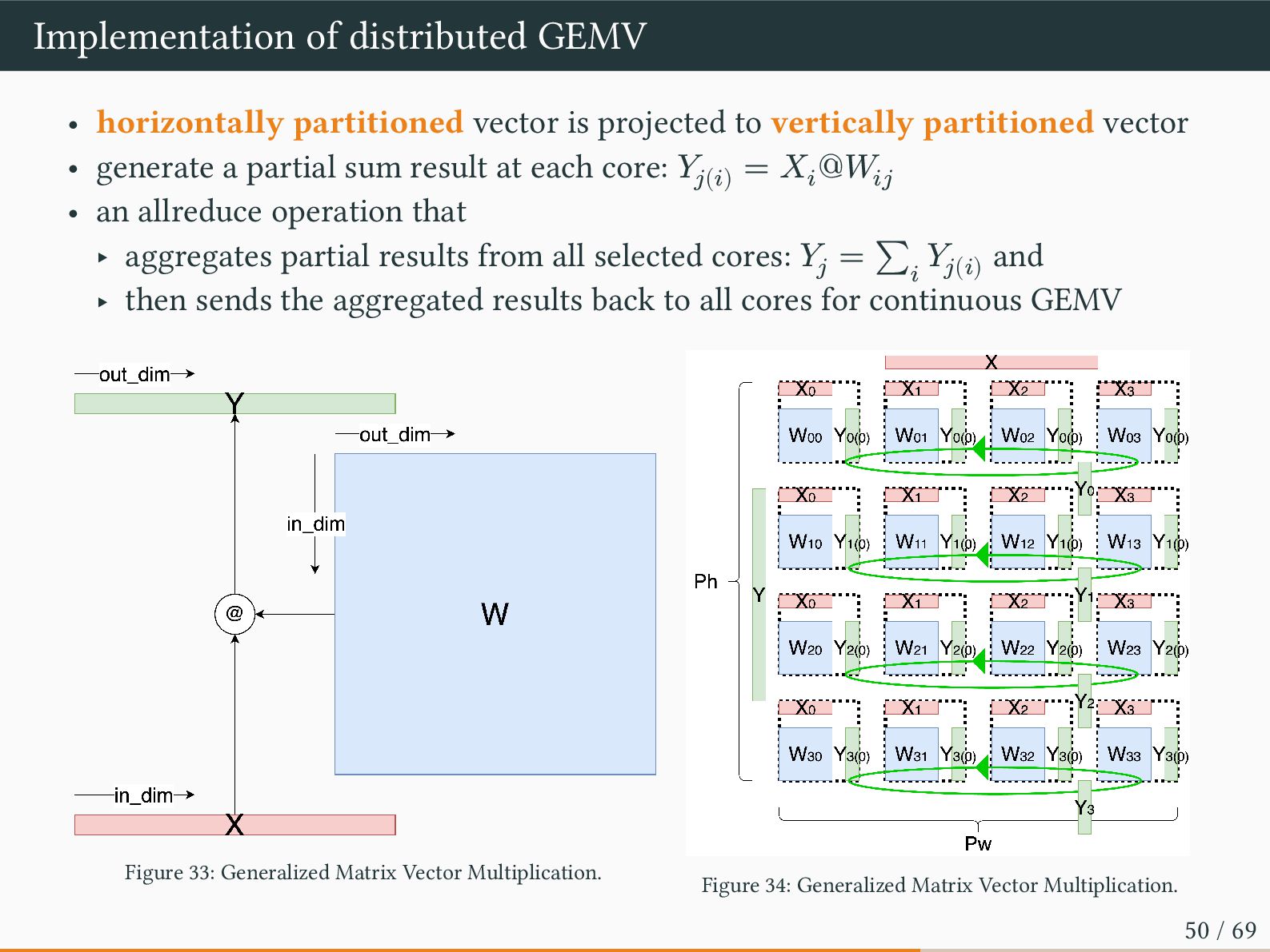
to vertically partitioned vector • generate a partial sum result at each core: 𝑌𝑗(𝑖) = 𝑋𝑖 @𝑊𝑖𝑗 • an allreduce operation that ‣ aggregates partial results from all selected cores: 𝑌𝑗 = ∑ 𝑖 𝑌𝑗(𝑖) and ‣ then sends the aggregated results back to all cores for continuous GEMV Figure 33: Generalized Matrix Vector Multiplication. Figure 34: Generalized Matrix Vector Multiplication. 50 / 69
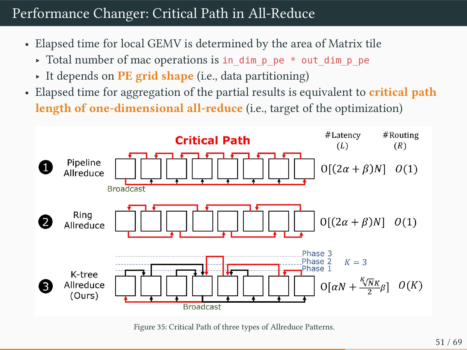
local GEMV is determined by the area of Matrix tile ‣ Total number of mac operations is in_dim_p_pe * out_dim_p_pe ‣ It depends on PE grid shape (i.e., data partitioning) • Elapsed time for aggregation of the partial results is equivalent to critical path length of one-dimensional all-reduce (i.e., target of the optimization) Figure 35: Critical Path of three types of Allreduce Patterns. 51 / 69
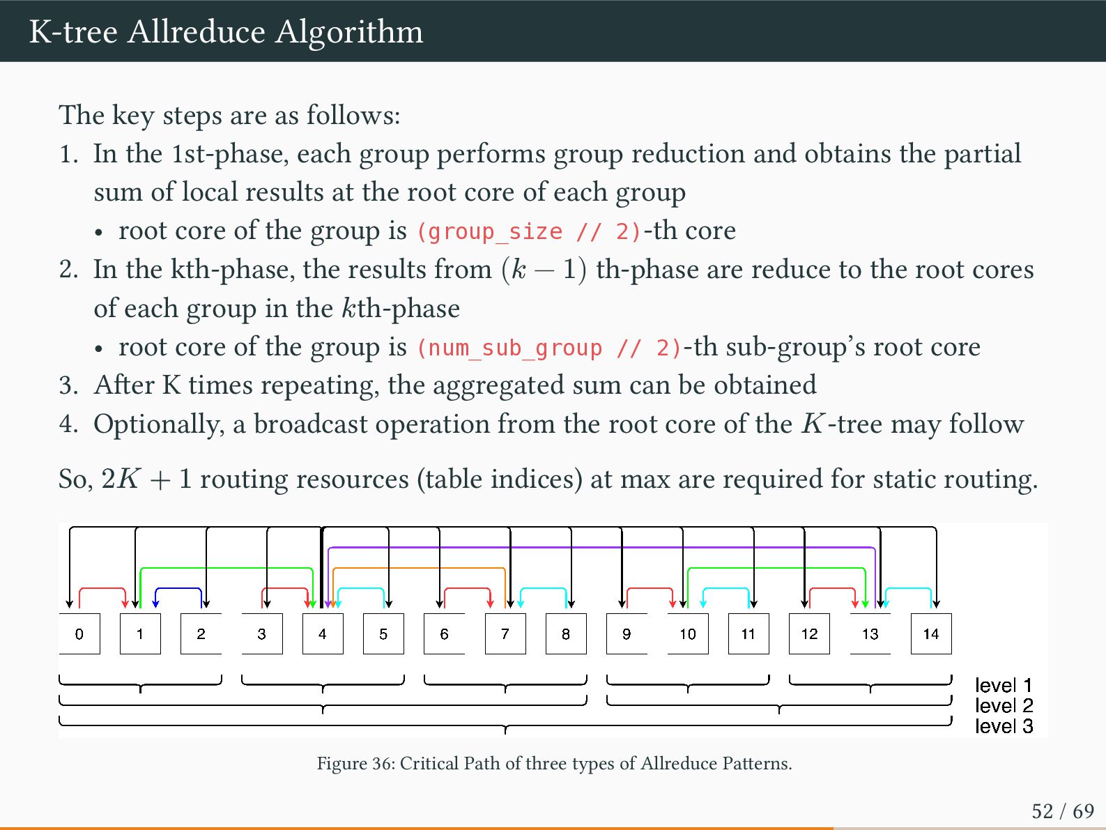
In the 1st-phase, each group performs group reduction and obtains the partial sum of local results at the root core of each group • root core of the group is (group_size // 2)-th core 2. In the kth-phase, the results from (𝑘 − 1) th-phase are reduce to the root cores of each group in the 𝑘th-phase • root core of the group is (num_sub_group // 2)-th sub-group’s root core 3. After K times repeating, the aggregated sum can be obtained 4. Optionally, a broadcast operation from the root core of the 𝐾-tree may follow So, 2𝐾 + 1 routing resources (table indices) at max are required for static routing. Figure 36: Critical Path of three types of Allreduce Patterns. 52 / 69
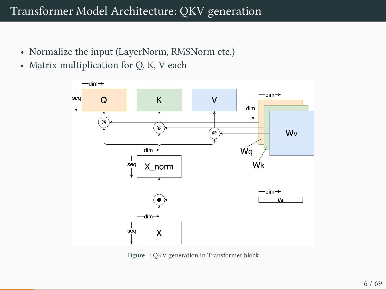
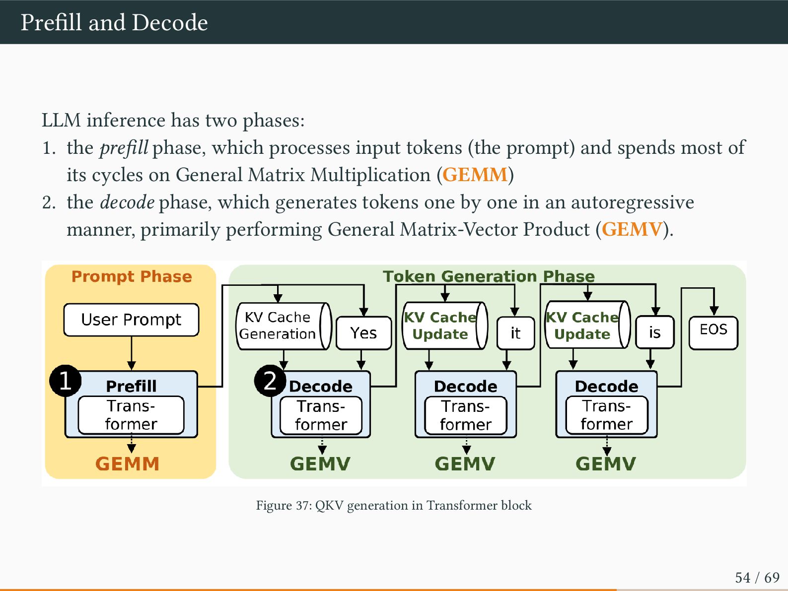
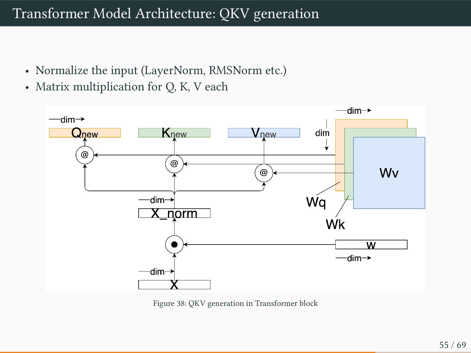
prefill phase, which processes input tokens (the prompt) and spends most of its cycles on General Matrix Multiplication (GEMM) 2. the decode phase, which generates tokens one by one in an autoregressive manner, primarily performing General Matrix-Vector Product (GEMV). Figure 37: QKV generation in Transformer block 54 / 69
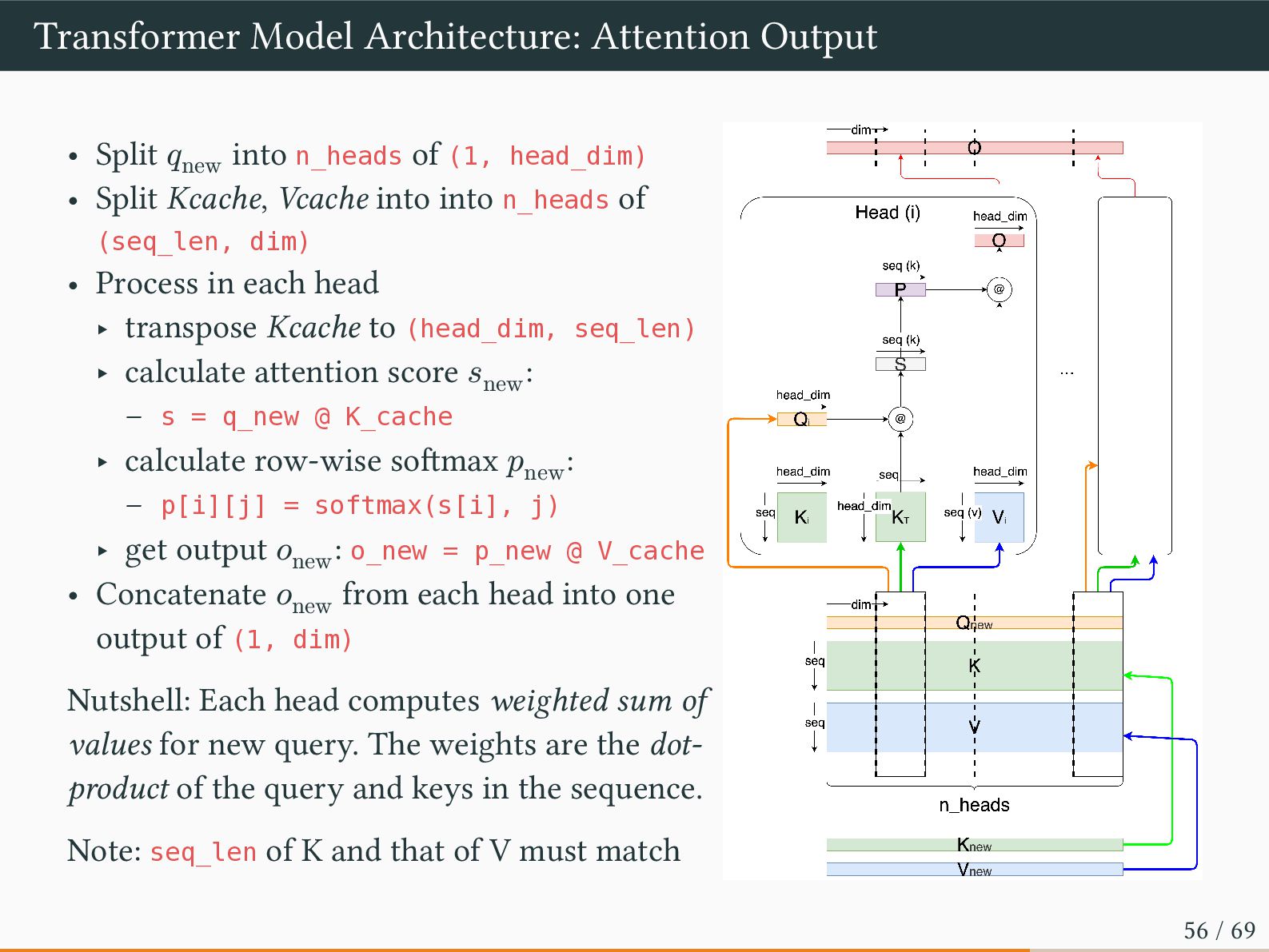
of (1, head_dim) • Split Kcache, Vcache into into n_heads of (seq_len, dim) • Process in each head ‣ transpose Kcache to (head_dim, seq_len) ‣ calculate attention score 𝑠new : – s = q_new @ K_cache ‣ calculate row-wise softmax 𝑝new : – p[i][j] = softmax(s[i], j) ‣ get output 𝑜new : o_new = p_new @ V_cache • Concatenate 𝑜new from each head into one output of (1, dim) Nutshell: Each head computes weighted sum of values for new query. The weights are the dot- product of the query and keys in the sequence. Note: seq_len of K and that of V must match 56 / 69
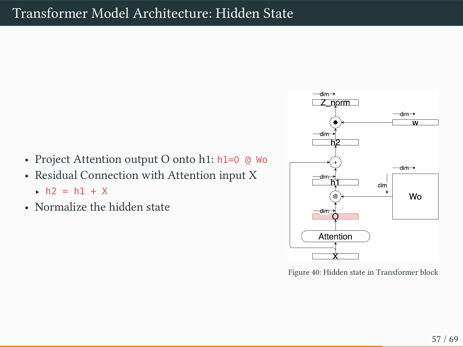
onto h1: h1=O @ Wo • Residual Connection with Attention input X ‣ h2 = h1 + X • Normalize the hidden state Figure 40: Hidden state in Transformer block 57 / 69
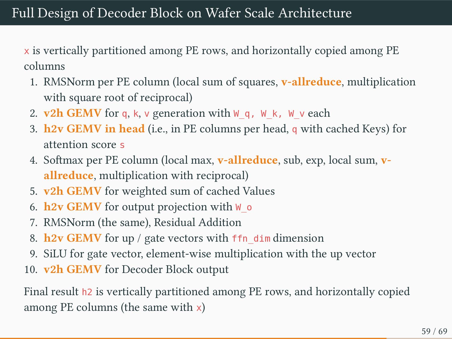
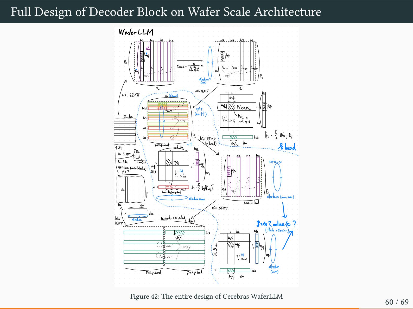
is vertically partitioned among PE rows, and horizontally copied among PE columns 1. RMSNorm per PE column (local sum of squares, v-allreduce, multiplication with square root of reciprocal) 2. v2h GEMV for q, k, v generation with W_q, W_k, W_v each 3. h2v GEMV in head (i.e., in PE columns per head, q with cached Keys) for attention score s 4. Softmax per PE column (local max, v-allreduce, sub, exp, local sum, v- allreduce, multiplication with reciprocal) 5. v2h GEMV for weighted sum of cached Values 6. h2v GEMV for output projection with W_o 7. RMSNorm (the same), Residual Addition 8. h2v GEMV for up / gate vectors with ffn_dim dimension 9. SiLU for gate vector, element-wise multiplication with the up vector 10. v2h GEMV for Decoder Block output Final result h2 is vertically partitioned among PE rows, and horizontally copied among PE columns (the same with x) 59 / 69
bsz bsz bsz bsz bsz bsz bsz bsz Wrms "/ "1dim 7 1 ~ ) copy ***X Knormi = dim orXnom Norm / dim copy Ph 1 allreduce Pr Pu ULL GEMT L bsZ U2h GEMT dim (dhead) ( Min/Pr bsz( j dim/Pul u :/// dimp & k WK , a , thij ⊥spit ) Wit ftn-dim bsz in W(k , ,+) px= = , py = I dim -- bsZ bsz = Wajj Ph bsZ & "I hZv GEMt dim (in head) Des-p-head head-dim * H b 121 -Ahead - hav GEMt z2 - bsz bsz bsz bsz - IRes Add Sin softmax 1///1 , 300h I & seg -Norm (vertical alreada " 1 /, 1008/4 Kathe ~ I it i I dim P M - head-dim/pes-p-head Preduce < (max , sum) 7 allreduce (sum) pes-p-head be VIh GEMT -dim I dim ↓ hav L n-heads + pe-p-head allreduce (= dim) GEMt EckZonline/t ? b (flash attention) i dim 11/IIII bsz dim/p Ora 11111 , 824:like u ↑ seg j Doe -Copy (N) seg Tiche allredree (sum) bsz pes-p-head pes-p-head = "dim Figure 42: The entire design of Cerebras WaferLLM 60 / 69
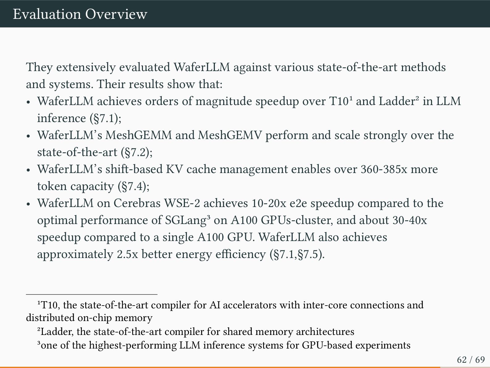
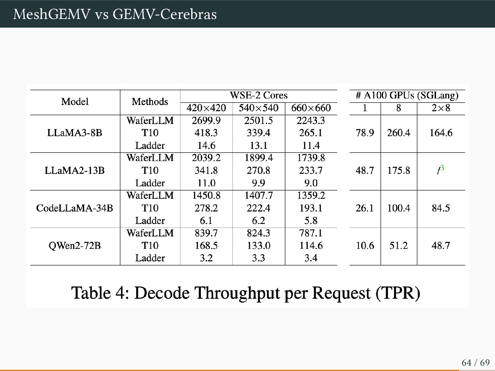
and systems. Their results show that: • WaferLLM achieves orders of magnitude speedup over T101 and Ladder2 in LLM inference (§7.1); • WaferLLM’s MeshGEMM and MeshGEMV perform and scale strongly over the state-of-the-art (§7.2); • WaferLLM’s shift-based KV cache management enables over 360-385x more token capacity (§7.4); • WaferLLM on Cerebras WSE-2 achieves 10-20x e2e speedup compared to the optimal performance of SGLang3 on A100 GPUs-cluster, and about 30-40x speedup compared to a single A100 GPU. WaferLLM also achieves approximately 2.5x better energy efficiency (§7.1,§7.5). 1T10, the state-of-the-art compiler for AI accelerators with inter-core connections and distributed on-chip memory 2Ladder, the state-of-the-art compiler for shared memory architectures 3one of the highest-performing LLM inference systems for GPU-based experiments 62 / 69
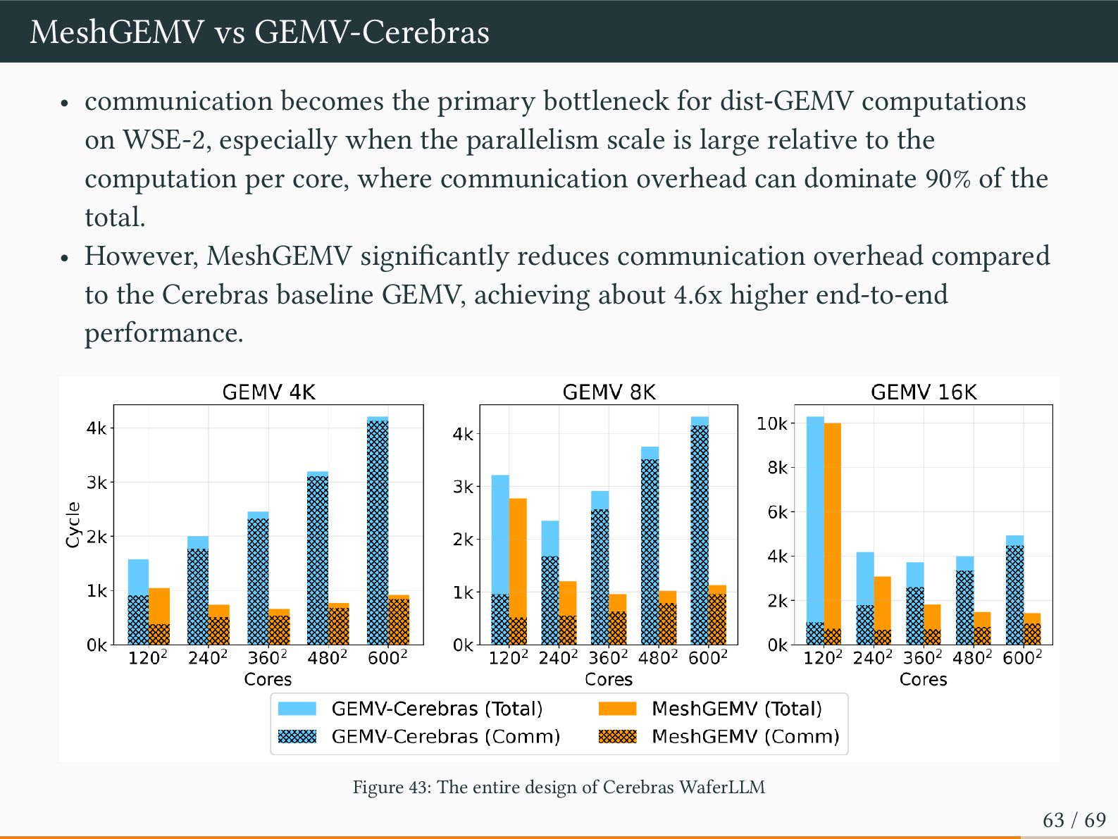
dist-GEMV computations on WSE-2, especially when the parallelism scale is large relative to the computation per core, where communication overhead can dominate 90% of the total. • However, MeshGEMV significantly reduces communication overhead compared to the Cerebras baseline GEMV, achieving about 4.6x higher end-to-end performance. Figure 43: The entire design of Cerebras WaferLLM 63 / 69
paper explicitly says something very suspicious: • Handles Prefill and decode transition: actually not, just adding the elapsed time of each • Uses offline autotuning to select core counts for each model: seems not, manually selected • supports variations of Self-Attention, including Grouped Query Attention, Multihead Attention: NO Paper reviewer will not examine your source code closely even in the artifact evaluation, but future researchers will inevitably notice this, and lies will always be exposed, so please stop. Exaggeration is always there, but false statements are distinct from exaggerations. 66 / 69
(max, +) and reduces memory accesses in Softmax calculation. • FlashAttention utilizes tiling for kernel fusion in order to reduce memory I/O regarding intermediate states • WaferLLM provides Prefill / Decode implementation on Cerebras Wafer Scale Engine for the first time with the Device model of Wafer Scale Architecture, focusing on reducing critical path length of 1D all-reduce 68 / 69


 gunnersgoestocl
 nttcom
 codmoninc
 recruitengineers
 techtekt
 minorun365
 greenmidori
 glaforge
 terapyon
 yamad
 camiha
 genda
 hiracky16
 sugarenia
 danielanewman
 chriscoyier
 szymonslowik
 swwweet
 uxyall
 rasagy
 vanstee
 jonyablonski
 nikkihalliwell
 addyosmani