Semantic Segmentation

Semantic Segmentation: Identify the object category of each pixel for every known object within an image. Labels are class-aware.

Transcript

1. Dissecting Semantic Segmentation By: Himanshu, Alfi Goyal, Rijesh Kumar, Jerin Joseph
2. Agenda 1. Motivation 2. Data Exploration 3. Architecture and Modeling 4. Evaluation 5. Results 2
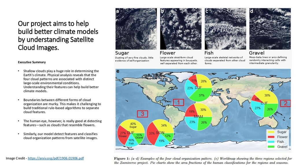
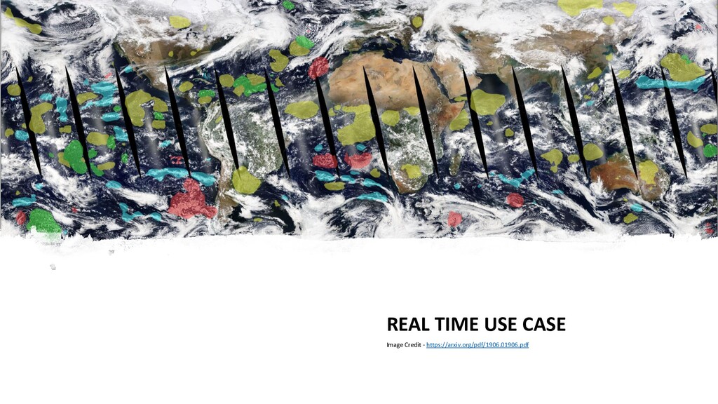
3. Our project aims to help build better climate models by understanding Satellite Cloud Images. Executive Summary • Shallow clouds play a huge role in determining the Earth's climate. Physical analysis reveals that the four cloud patterns are associated with distinct large-scale environmental conditions. Understanding their features can help build better climate models. • Boundaries between different forms of cloud organization are murky. This makes it challenging to build traditional rule-based algorithms to separate cloud features. • The human eye, however, is really good at detecting features—such as clouds that resemble flowers. • Similarly, our model detect features and classifies cloud organization patterns from satellite images. Image Credit - https://arxiv.org/pdf/1906.01906.pdf
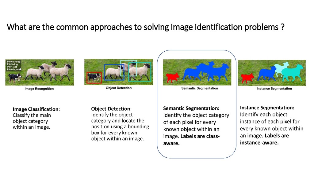
4. What are the common approaches to solving image identification problems ? Object Detection: Identify the object category and locate the position using a bounding box for every known object within an image. Semantic Segmentation: Identify the object category of each pixel for every known object within an image. Labels are class- aware. Instance Segmentation: Identify each object instance of each pixel for every known object within an image. Labels are instance-aware. Image Classification: Classify the main object category within an image.
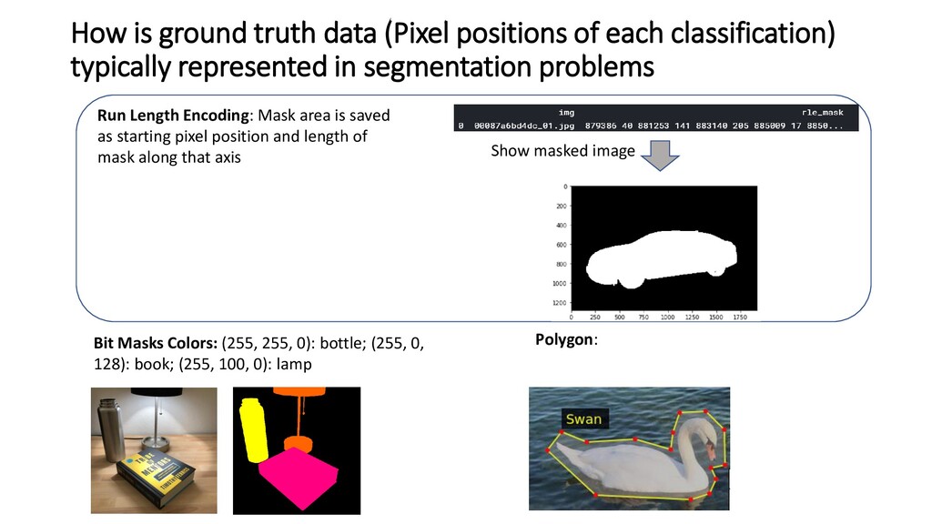
5. How is ground truth data (Pixel positions of each classification) typically represented in segmentation problems Run Length Encoding: Mask area is saved as starting pixel position and length of mask along that axis Bit Masks Colors: (255, 255, 0): bottle; (255, 0, 128): book; (255, 100, 0): lamp Polygon: Show masked image
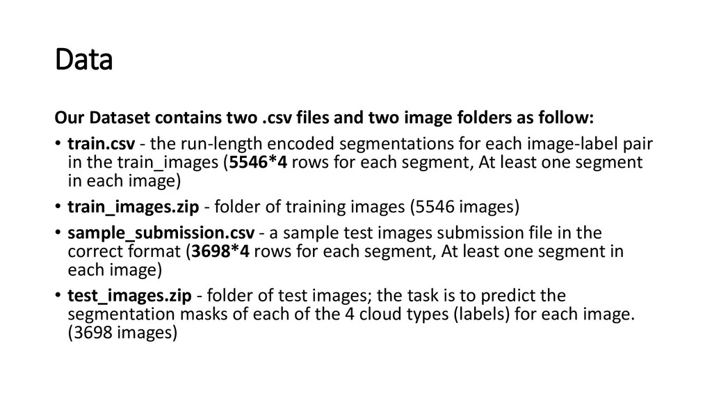
6. Data Our Dataset contains two .csv files and two image folders as follow: • train.csv - the run-length encoded segmentations for each image-label pair in the train_images (5546*4 rows for each segment, At least one segment in each image) • train_images.zip - folder of training images (5546 images) • sample_submission.csv - a sample test images submission file in the correct format (3698*4 rows for each segment, At least one segment in each image) • test_images.zip - folder of test images; the task is to predict the segmentation masks of each of the 4 cloud types (labels) for each image. (3698 images)
7. Training Data Shape
8. Number of Cloud Types per Image and Frequency of different clouds
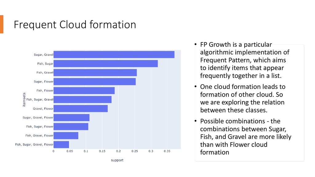
9. Frequent Cloud formation • FP Growth is a particular algorithmic implementation of Frequent Pattern, which aims to identify items that appear frequently together in a list. • One cloud formation leads to formation of other cloud. So we are exploring the relation between these classes. • Possible combinations - the combinations between Sugar, Fish, and Gravel are more likely than with Flower cloud formation
10. Surface Area Ratio Per Cloud Formation
11. Visualizing Training labels
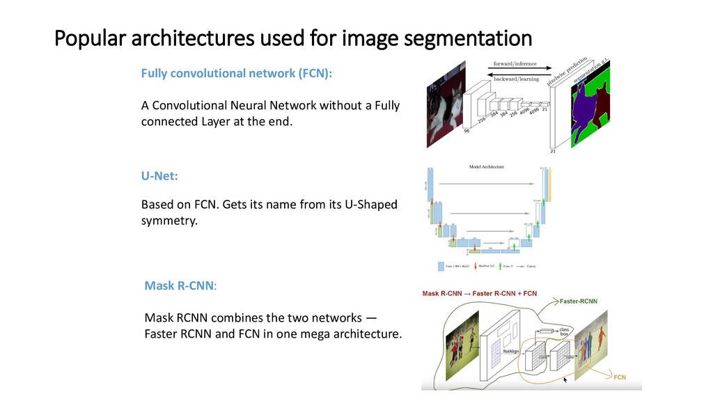
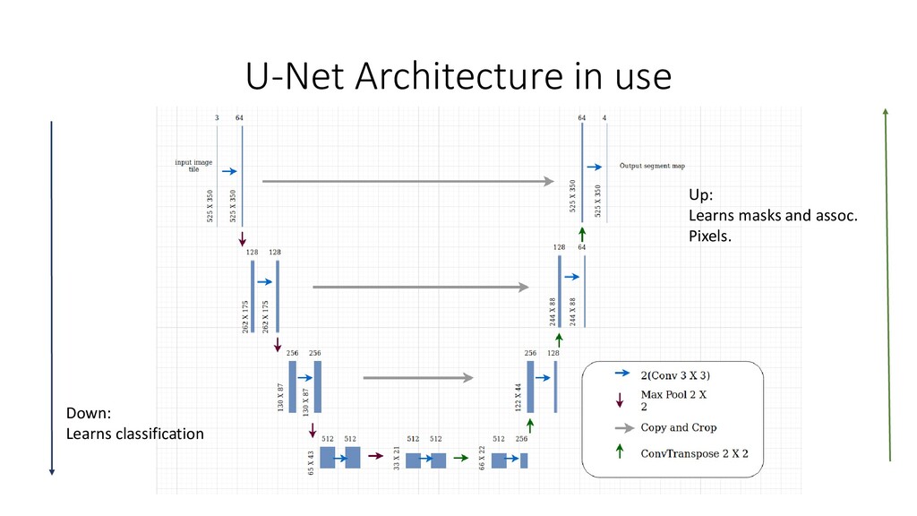
12. Popular architectures used for image segmentation Fully convolutional network (FCN): A Convolutional Neural Network without a Fully connected Layer at the end. U-Net: Based on FCN. Gets its name from its U-Shaped symmetry. Mask R-CNN: Mask RCNN combines the two networks — Faster RCNN and FCN in one mega architecture.
13. U-Net Architecture in use Down: Learns classification Up: Learns masks and assoc. Pixels.
14. Training: Parameters • # of Epochs : 32, 1 - Fold • Evaluation: Dice score (More on it next) • Total time taken: ~6 Hours • Optimizer: RAdam (Rectified Adam) • Loss Function – BCE (Classification) + Dice (Segmentation) • Data Transformation • Albumentation library: (Augmentation) • Horizontal flip | shift scale rotate | distort | resize | normalize • Regularization - Learning Rate Decay
15. Training: Plots
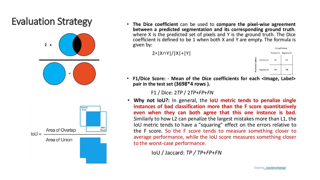
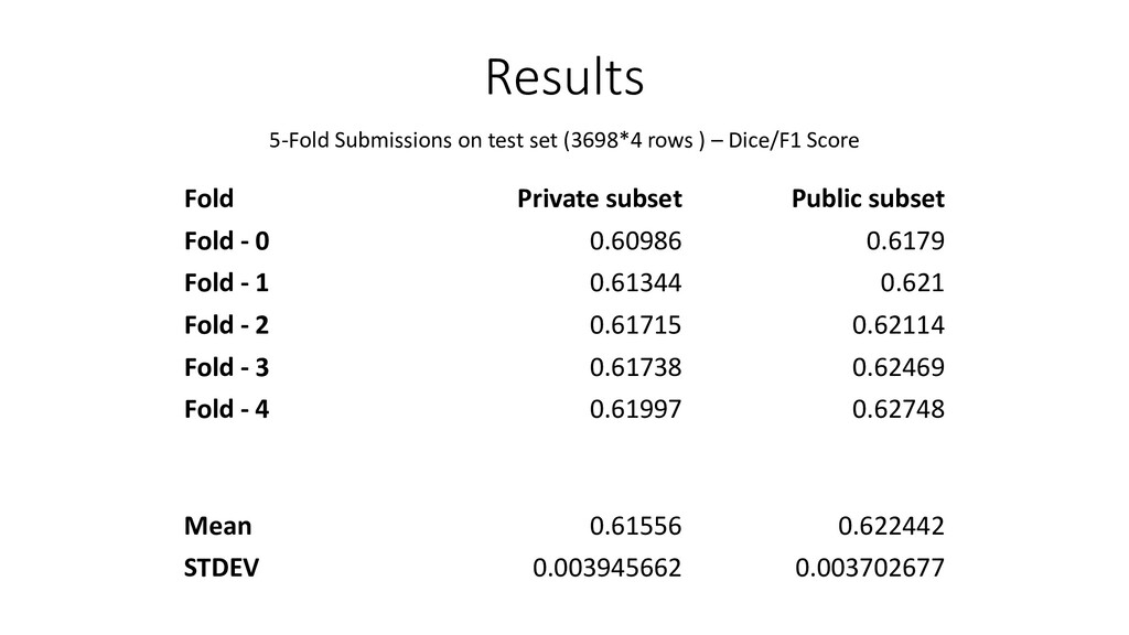
16. • The Dice coefficient can be used to compare the pixel-wise agreement between a predicted segmentation and its corresponding ground truth. where X is the predicted set of pixels and Y is the ground truth. The Dice coefficient is defined to be 1 when both X and Y are empty. The formula is given by: 2∗|X∩Y|/|X|+|Y| • F1/Dice Score: - Mean of the Dice coefficients for each <Image, Label> pair in the test set (3698*4 rows ). F1 / Dice: 2TP / 2TP+FP+FN Evaluation Strategy Source: stackexchange • Why not IoU?: In general, the IoU metric tends to penalize single instances of bad classification more than the F score quantitatively even when they can both agree that this one instance is bad. Similarly to how L2 can penalize the largest mistakes more than L1, the IoU metric tends to have a "squaring" effect on the errors relative to the F score. So the F score tends to measure something closer to average performance, while the IoU score measures something closer to the worst-case performance. IoU / Jaccard: TP / TP+FP+FN
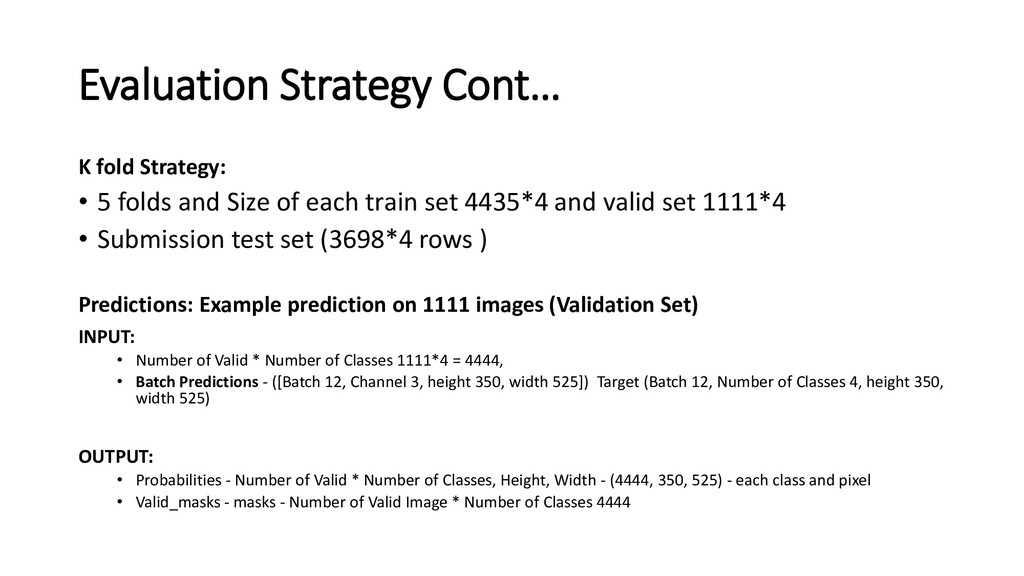
17. Evaluation Strategy Cont… K fold Strategy: • 5 folds and Size of each train set 4435*4 and valid set 1111*4 • Submission test set (3698*4 rows ) Predictions: Example prediction on 1111 images (Validation Set) INPUT: • Number of Valid * Number of Classes 1111*4 = 4444, • Batch Predictions - ([Batch 12, Channel 3, height 350, width 525]) Target (Batch 12, Number of Classes 4, height 350, width 525) OUTPUT: • Probabilities - Number of Valid * Number of Classes, Height, Width - (4444, 350, 525) - each class and pixel • Valid_masks - masks - Number of Valid Image * Number of Classes 4444
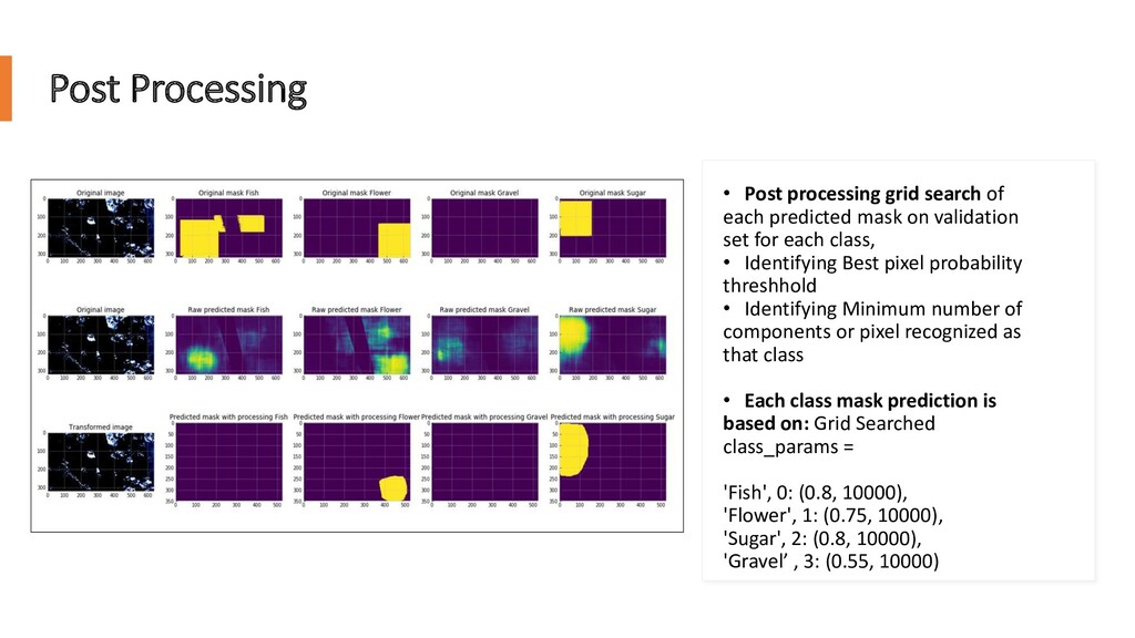
18. Post Processing • Post processing grid search of each predicted mask on validation set for each class, • Identifying Best pixel probability threshhold • Identifying Minimum number of components or pixel recognized as that class • Each class mask prediction is based on: Grid Searched class_params = 'Fish', 0: (0.8, 10000), 'Flower', 1: (0.75, 10000), 'Sugar', 2: (0.8, 10000), 'Gravel’ , 3: (0.55, 10000)
19. Results 5-Fold Submissions on test set (3698*4 rows ) – Dice/F1 Score Fold Private subset Public subset Fold - 0 0.60986 0.6179 Fold - 1 0.61344 0.621 Fold - 2 0.61715 0.62114 Fold - 3 0.61738 0.62469 Fold - 4 0.61997 0.62748 Mean 0.61556 0.622442 STDEV 0.003945662 0.003702677
20. Test Set Mask Output (Original, Predicted Mask, Predicted Convex Hull Post Processed Mask) • Blue- Sugar • White – Gravel • Green – Flower • Red – Fish
21. REAL TIME USE CASE Image Credit - https://arxiv.org/pdf/1906.01906.pdf
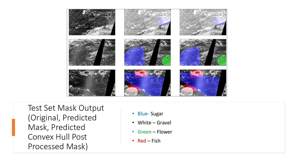
22. What we learned? Advantage: • Unet – Very Simple Model Architecture performs well on segmentation. Helped us understand various stages of semantic segmentation. • Submissions results on test set(3698*4 rows) shows up Models generalizability which is acceptable. Disadvantage: • Classification ensemble would have helped gain better dice score since the submission mask was for each class. (Instead of Post Processing) • Very Simple Segmentation Architecture – Mask RCNN could do better at making right mask predictions Future Work: • Fine Tuning more complex models • Re-Evaluating model performance (Including new regularization parameters(such as Dropout) and augmentation tricks) • Experiment new methods – Detectron2 Mask RCNN Transfer Learning (Which we had no success implementing) 22
23. References • https://www.kaggle.com/dhananjay3/image-segmentation-from-scratch-in-pytorch - Finally Huge thanks to Dhananjay, artgor, ryches, ratthachat, repo1 ,repo2 for their code • https://www.kaggle.com/artgor/segmentation-in-pytorch-using-convenient-tools • https://www.kaggle.com/ryches/turbo-charging-andrew-s-pytorch • https://github.com/qubvel/segmentation_models.pytorch/blob/master/segmentation _models_pytorch/utils/losses.py • https://github.com/milesial/Pytorch-UNet • https://www.kaggle.com/ratthachat/cloud-convexhull-polygon-postprocessing-no-gpu • https://www.analyticsvidhya.com/blog/2019/07/computer-vision-implementing-mask- r-cnn-image-segmentation/ • https://medium.com/@jonathan_hui/map-mean-average-precision-for-object- detection-45c121a31173 • https://stats.stackexchange.com/questions/195006/is-the-dice-coefficient-the-same- as-accuracy