Inferences about process quality

INFERENCES ABOUT PROCESS QUALITY
— Based on D. C. Montgomery’s Statistical Quality Control —
H. Kemal İlter, PhD
F
@hkilter
January 2020

View Slide

WELCOME
About Me
H. Kemal İlter, PhD
Associate Professor of Operations Management
Visiting Researcher
ENCS Concordia University
www.hkilter.com
[email protected]
[email protected]
Contents
1. Introduction
2. Statistics and Sampling Distributions
3. Point Estimation of Process Parameters
4. Statistical Inference for a Single Sample
5. Statistical Inference for Two Samples

View Slide

PARAMETERS, KNOWN OR UNKNOWN?
Unrealistic assumption
In the use of probability distributions in modeling or
describing the output of a process, we assumed that the
parameters of the probability distribution, and, hence, the
parameters of the process, are known.
For example, in using the binomial distribution to model the
number of defective items found in sampling from a
production process we assumed that the parameter p of the
binomial distribution is known.
The physical interpretation of p is that it is the true fraction of
defective items produced by the process.
It is impossible to know this exactly in a real production
process. Furthermore, if we know the true value of p and it is
relatively constant over time, we can argue that formal process
monitoring and control procedures are unnecessary, provided
p is acceptably small.

View Slide

PARAMETERS, KNOWN OR UNKNOWN?
In general, the parameters of a process are unknown;
furthermore, they can usually change over time.
Therefore, we need to develop procedures to;
▶ estimate the parameters of probability distributions, and
▶ solve inference or decision-oriented problems
These techniques are the underlying basis for much of the
methodology of statistical quality control.

View Slide

INFERENCE
The name inferential statistics derives from the term
inference, given definition by the Merriam-Webster online
dictionary*:
the act of passing from statistical sample data to
generalizations (as of the value of population parameters)
usually with calculated degrees of certainty
Inference is a method of making suppositions about an
unknown, drawing on what is known to be true.
* https://www.merriam-webster.com/dictionary/inference

View Slide

STATISTICAL INFERENCE
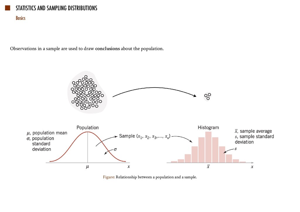
Statistical inference is a process of making generalizations
about unmeasured populations using data calculated on
measured samples.
Statistical inference has the advantage of quantifying the
degree of certainty for a particular inference.
People sometimes get confused about the difference between
descriptive statistics and inferential statistics, partly because
in many cases the statistical procedures used are identical while
the interpretation differs.
Basic rule
Any time you want to generalize your results beyond the
specific cases that provided your data, you should be doing
inferential statistics.

View Slide

STATISTICS AND SAMPLING DISTRIBUTIONS
Basics
Observations in a sample are used to draw conclusions about the population.
Figure: Relationship between a population and a sample.

View Slide

Sampling
Sampling
The process of defining the population and selecting an
appropriate sampling method can be quite complex.
Nonprobability Sampling (highly subject to sampling bias)
▶ Volunteer sampling
▶ Convenience sampling
▶ Quota sampling
Probability Sampling
▶ Simple random sampling
▶ Systematic sampling
▶ Complex random sampling (stratified sampling, cluster
sampling)
Random sampling
Random samples drawn from;
▶ infinite populations
▶ finite populations with replacement
▶ finite populations without replacement
Randomness
Random behavior a.k.a randomness comes from;
▶ the environment (eg. Brownian motion)
▶ the initial conditions (eg. Chaos theory)
▶ generated by the system, pseudorandomness
(Pseudo-random number generators)

View Slide

.

View Slide

Statistic
Statistic is any function of the sample data that does not
contain unknown parameters.
Let x1
, x2
, . . . , xn
represent the observations in a sample.
The sample mean
¯
x =
∑
n
i=1
xi
n
the sample variance
s2 =
∑
n
i=1
(xi
− ¯
x)2
n − 1
and, the sample standard deviation
s =
√∑
n
i=1
(xi
− ¯
x)2
n − 1
are statistics. The statistics ¯
x and s (or s2 ) describe the central
tendency and variability, respectively, of the sample.
A statistic is a random variable, because a different sample will
produce a different observed value of the statistic.
Every statistic has a probability distribution.
If we know the probability distribution of the population from
which the sample was taken, we can often determine the
probability distribution of various statistics computed from the
sample data. The probability distribution of a statistic is called
a sampling distribution.
When a statistic is used to estimate a population parameter, is
called an estimator.
It can be proved that the mean of a sample is an unbiased
estimator of the population mean. This means that the
average of multiple sample means will tend to converge to the
true mean of the population.

View Slide

EFFECT OF THE SAMPLE SIZE
Figure: Histogram of a uniformly distributed
population (N = 100) with range 0 − 100.
Figure: Distribution of the means of 100 samples of
size n = 2, drawn from a uniform distribution.
Figure: Distribution of means of 100 samples of size
n = 25, drawn from a uniform distribution.

View Slide

Sampling Distributions
Sampling distributions are important in statistics because they
provide a major simplification en route to statistical inference.
More specifically, they allow analytical considerations to be
based on the probability distribution of a statistic, rather than
on the joint probability distribution of all the individual sample
values.
Figure: Many sample observations (black) are shown from a joint
probability distribution.

View Slide

Sampling from a Normal Distribution
Suppose that x is a normally distributed random variable with
mean µ and variance σ2. If x1
, x2
, . . . , xn
is a random sample of
size n from this process, then the distribution of the sample
mean
¯
x = N(µ, σ2/n)
From the central limit theorem we know that, regardless of the
distribution of the population, the distribution of
∑
u
i=1
xi
is
approximately normal with mean nµ and variance nσ2.
Therefore, regardless of the distribution of the population, the
sampling distribution of the sample mean is approximately
¯
x ∼ N(µ,
σ2
n
)
So, the mean of x is approximately normally distributed with
mean µ and variance σ2/n.

View Slide

Chi-square or χ2 distribution
Suppose that a random sample of n
observations — say, x1
, x2
, . . . , xn
— is
taken from a chi-square or χ2
distribution with mean zero and variance
one. Then the random variable
y = x2
1
+ x2
2
+ · · · + x2
n
has a chi-square or χ2 distribution with
n degrees of freedom.
Figure: Chi-square distribution for selected values
of n (number of degrees of freedom).
t distribution
If x is a standard normal random variable
and if y is a chi-square random variable
with k degrees of freedom, and if x and y
are independent, then the random
variable
t =
x
√
y
k
is distributed as t with k degrees of
freedom.
Figure: The t distribution for selected values of k
(number of degrees of freedom).
F distribution
If w and y are two independent chi-square
random variables with u and v degrees of
freedom, respectively, then the ratio
Fu,v
=
w/u
y/v
is distributed as F with u numerator
degrees of freedom and v denominator
degrees of freedom.
Figure: The F distribution for selected values of u
(numerator degrees of freedom).

View Slide

Chi-square or χ2 distribution t distribution F distribution

View Slide

Sampling from a Bernoulli Distribution
Suppose that a random sample of n observations — say,
x1
, x2
, . . . , xn
— is taken from a Bernoulli process with constant
probability of success p. Then the sum of the sample
observations
x = x1
+ x2
+ · · · + xn
has a binomial distribution with parameters n and p.
Furthermore, since each xi
is either 0 or 1, the sample mean
¯
x =
1
n
n
∑
i=1
xi
is a discrete random variable with range space
{0, 1/n, 2/n, . . . , (n − 1)/n, 1}. The distribution of ¯
x can be
obtained from the binomial since
P{¯
x ≤ a} = P{¯
x ≤ an} =
[an]
∑
k=0
(
n
k
)
pk(1 − p)(n − k)
where [an] is the largest integer less than or equal to an. The
mean and variance of ¯
x are
µ¯
x
= p
and
σ2
¯
x
=
p(1 − p)
n
respectively.

View Slide

Sampling from a Poisson Distribution
Suppose that a random sample of n observations — say,
x1
, x2
, . . . , xn
— is taken from a Poisson distribution with
parameter λ. Then the sum of the sample observations
x = x1
+ x2
+ · · · + xn
has a Poisson distribution with parameter nλ.
¯
x =
1
n
n
∑
i=1
xi
is a discrete random variable with range space
{0, 1/n, 2/n, . . . }. The distribution of ¯
x can be obtained from
P{¯
x ≤ a} = P{¯
x ≤ an} =
[an]
∑
k=0
e−nλ(nλ)k
k!
where [an] is the largest integer less than or equal to an. The
mean and variance of ¯
x are
µ¯
x
= λ
and
σ2
¯
x
=
λ
n

View Slide

POINT ESTIMATION OF PROCESS PARAMETERS
The techniques of statistical inference can be classified into two
broad categories: parameter estimation and hypothesis testing.
Distributions are described by their parameters.
Parameters are generally unknown and must be estimated.
Point estimator is a statistic that a single numerical value that
is the estimate of the parameter.
Properties
1. The point estimator should be unbiased. That is, the
expected value of the point estimator should be the
parameter being estimated.
2. The point estimator should have minimum variance.
Any point estimator is a random variable. Thus, a
minimum variance point estimator should have a variance
that is smaller than the variance of any other point
estimator of that parameter.
In many applications of statistics to quality-engineering
problems, it is convenient to estimate the standard deviation by
the range method.
The range of the sample is
R = max(xi
) − min(xi
) = xmax
− xmin
The random variable W = R/σ is called the relative range.
The mean of W is a constant d2
that depends on the size of the
sample. That is, E(W) = d2
.
Therefore, an unbiased estimator of the standard deviation σ of
a normal distribution is
ˆ
σ =
R
d2
Values of d2
for sample sizes 2 ≤ n ≤ 25 are given in the
Appendix Table VI.

View Slide

STATISTICAL HYPOTHESIS
Basics
A statistical hypothesis is a statement about the values of the
parameters of a probability distribution.
For example, suppose we think that the mean inside diameter
of a bearing is 1.500 in. We may express this statement in a
formal manner as
H0
: µ = 1.500
H1
: µ ̸= 1.500
The statement H0
: µ = 1.500 is called the null hypothesis,
and H1
: µ ̸= 1.500 is called the alternative hypothesis.
In the example, H1
specifies values of the mean diameter that
are either greater than 1.500 or less than 1.500, and is called a
two-sided alternative hypothesis. Depending on the problem,
various one-sided alternative hypotheses may be appropriate.
An important part of any hypothesis testing problem is
determining the parameter values specified in the null and
alternative hypotheses.
1. The values may result from past evidence or knowledge.
This happens frequently in statistical quality control,
where we use past information to specify values for a
parameter corresponding to a state of control, and then
periodically test the hypothesis that the parameter value
has not changed.
2. The values may result from some theory or model of the
process.
3. The values chosen for the parameter may be the result of
contractual or design specifications, a situation that occurs
frequently.

View Slide

Hypothesis Testing
To test a hypothesis, we take a random sample from the
population under study, compute an appropriate test statistic,
and then either reject or fail to reject the null hypothesis H0
.
The set of values of the test statistic leading to rejection of H0
is
called the critical region or rejection region for the test.
Two kinds of errors may be committed when testing
hypotheses.
▶ If the null hypothesis is rejected when it is true, then a
type I error has occurred.
▶ If the null hypothesis is not rejected when it is false, then a
type II error has been made.
The probabilities of these two types of errors are denoted as
α = P{ type I error } = P{ reject H0
|H0
is true }
β = P{ type II error } = P{ fail to reject H0
|H0
is false }
Sometimes it is more convenient to work with the power of a
statistical test, where
Power = 1 − β = P{ reject H0
|H0
is false }
Thus, the power is the probability of correctly rejecting H0
.
In quality control work, α is sometimes called the producer’s
risk, because it denotes the probability that a good lot will be
rejected, or the probability that a process producing acceptable
values of a particular quality characteristic will be rejected as
performing unsatisfactorily.
In addition, β is sometimes called the consumer’s risk, because
it denotes the probability of accepting a lot of poor quality, or
allowing a process that is operating in an unsatisfactory manner
relative to some quality characteristic to continue in operation.

View Slide

Figure: Type I and Type II errors.

View Slide

CONFIDENCE INTERVALS
When we calculate a single statistic, such as the mean, to
describe a sample, that is referred to as calculating a point
estimate because the number represents a single point on the
number line. The sample mean is a point estimate, and is a
useful statistic as the best estimate of the population mean.
However, we know that the sample mean is only an estimate
and that if we drew a different sample, the mean of the sample
would probably be different. We don’t expect that every
possible sample we could draw will have the same sample mean.
It is reasonable to ask how much the point estimate is likely to
vary by chance if we had chosen a different sample, and in
many professional fields it has become common practice to
report both point estimates and interval estimates. A point
estimate is a single number, while an interval estimate is a
range or interval of numbers.
The most common interval estimate is the confidence interval,
which is the interval between two values that represent the
upper and lower confidence limits or confidence bounds for a
statistic. The formula used to calculate the confidence interval
depends on the statistic being used. The confidence interval is
calculated using a predetermined significance level, often called
α, which is most often set at 0.05, as discussed above. The
confidence coefficient is calculated as (1 − α) or, as a
percentage, 100(1 − α)%. Thus if α = 0.05, the confidence
coefficient is 0.95 or 95%.
Confidence intervals are based on the notion that if a study was
repeated an infinite number of times, each time drawing a
different sample from the same population and constructing a
confidence interval based on that sample, x% of the time the
confidence interval would contain the unknown parameter
value that the study seeks to estimate.
The confidence interval conveys important information about
the precision of the point estimate.

View Slide

CONFIDENCE INTERVALS
An interval estimate of a parameter is the interval between two
statistics that includes the true value of the parameter with
some probability. For example, to construct an interval
estimator of the mean m, we must find two statistics L and U
such that
P{L ≤ µ ≤ U} = 1 − α
The resulting interval
L ≤ µ ≤ U
is called a 100(1 − α)% confidence interval for the unknown
mean µ. L and U are called the lower and upper confidence
limits, respectively, and 1 − a is called the confidence
coefficient. Sometimes the half-interval width U − m or m − L
is called the accuracy of the confidence interval. The
interpretation of a CI is that if a large number of such intervals
are constructed, each resulting from a random sample, then
100(1 − α)% of these intervals will contain the true value of µ.
Thus, confidence intervals have a frequency interpretation.

View Slide

P-VALUE
The traditional way to report the results of a hypothesis test is
to state that the null hypothesis was or was not rejected at a
specified α-value or level of significance.
The P-value is the smallest level of significance that would lead
to rejection of the null hypothesis H0
.
Once the P-value is known, the decision maker can determine
for himself or herself how significant the data are without the
data analyst formally imposing a preselected level of
significance.

View Slide

P-VALUE
Figure: P-value (Source: https://xkcd.com/1478/).

View Slide

INFERENCE FOR ONE SAMPLE
Mean of a Population, Variance Known
x is a random variable with unknown mean µ and known
variance σ2. Test the hypothesis that the mean is equal to a
standard value, µ0
.
Hypotheses
H0
: µ = µ0
H1
: µ ̸= µ0
Procedure
1. Take a random sample of n observations on the random
variable x,
2. Compute the test statistic, Z0
,
Z0
=
¯
x − µ0
σ/
√
n
3. Reject H0
if |Z0
| > Zα/2
where Zα/2
is the upper α/2
percentage point of the standard normal distribution.

View Slide

INFERENCE
Mean of a Population, Variance Known
Example
The response time of a distributed computer system is an
important quality characteristic. The system manager wants to
know whether the mean response time to a specific type of
command exceeds 75 millisec. From previous experience, he
knows that the standard deviation of response time is 8 mil-
lisec. Use a type I error of α = 0.05.
Solution
H0
: µ = 75
H1
: µ > 75
The command is executed 25 times and the response time for
each trial is recorded. We assume that these observations can
be considered as a random sample of the response times. The
sample average response time is ¯
x = 79.25 millisec. The value
of the test statistic is
Z0
=
¯
x − µ0
σ/
√
n
=
79.25 − 75
8
√
25
= 2.66
Because we specified a type I error of α = 0.05 and the test is
one-sided, then from Appendix Table II we find
Zα
= Z0.05
= 1.645. Therefore, we reject H0
: µ = 75 and
conclude that the mean response time exceeds 75 millisec.
Since ¯
x = 79.25 millisec, we know that a reasonable point
estimate of the mean response time is ˆ
µ = ¯
x = 79.25 millisec.
Find a 95% two-sided confidence interval.
¯
x − Zα/2
σ
√
n
≤ µ ≤ ¯
x + Zα/2
σ
√
n
79.25 − 1.96
8
√
25
≤ µ ≤ 79.25 + 1.96
8
√
25
76.114 ≤ µ ≤ 82.386
Another way to express this result is that our estimate of mean
response time is 79.25 millisec ± 3.136 millisec with 95%
confidence.

View Slide

INFERENCE
Mean of a Population, Variance Unknown
x is a random variable with unknown mean µ and unknown
variance σ2. Test the hypothesis that the mean is equal to a
standard value, µ0
.
Hypotheses
H0
: µ = µ0
H1
: µ ̸= µ0
Procedure
variable x,
2. Compute the test statistic, t0
. As σ2 is unknown, it may be
estimated by s2. If we replace σ by s, we have the test
statistic
t0
=
¯
x − µ0
s/
√
n
3. Reject H0
if |t0
| > tα/2,n−1
where tα/2,n−1
is the upper α/2
percentage point of the t distribution with n − 1 degrees
freedom.

View Slide

INFERENCE
Example
Rubber can be added to asphalt to reduce road noise when the
material is used as pavement. Table shows the stabilized
viscosity (cP) of 15 specimens of asphalt paving material. To be
suitable for the intended pavement application, the mean
stabilized viscosity should be equal to 3200. Test this
hypothesis using α = 0.05. Based on experience we are willing
to initially assume that stabilized viscosity is normally
distributed.
Figure: Stabilized viscosity of rubberized asphalt.
Solution
Hypothesis
H0
: µ = 3200
H1
: µ ̸= 3200
Sample mean
¯
x =
1
15
15
∑
i=1
xi
=
48161
15
= 3210.73
Sample standard deviation
s =
√
∑
15
i=1
x2
i
− (
∑
15
i=1
xi)2
15
15 − 1
=
√
154825783 − (48161)2
15
14
= 117.61
Test statistic
t0
=
¯
x − µ0
s/
√
n
=
3210.73 − 3200
117.61
√
15
= 0.35

View Slide

INFERENCE
Solution (cont.)
Since the calculated value of the test statistic does not exceed
t0.025,14
= 2.145 or − t0.025,14
= −2.145, we cannot reject the
null hypothesis. Therefore, there is no strong evidence to
conclude that the mean stabilized viscosity is different from
3200 cP.
The assumption of normality for the t-test can be checked by
constructing a normal probability plot of the stabilized
viscosity data. Figure shows the normal probability plot.
Because the observations lie along the straight line, there is no
problem with the normality assumption.
Figure: Normal probability plot of the stabilized viscosity data.
Find a 95% confidence interval on the mean stabilized viscosity.
¯
x − tα/2,n−1
s
√
n
≤ µ ≤ ¯
x + tα/2,n−1
s
√
n
3210.73 − 2.145
117.61
√
15
≤ µ ≤ 3210.73 + 2.145
117.61
√
15
3145.59 ≤ µ ≤ 3275.87
Another way to express this result is that our estimate of mean
response time is 3210.73 cP ± 65.14 cP with 95% confidence.
The manufacturer may only be concerned about stabilized
viscosity values that are too low and consequently may be
interested in a one-sided confidence bound. The 95% lower
confidence bound on mean stabilized viscosity is found using
t0.05,14
= 1.761 as
3210.73 − 1.761
117.61
√
15
≤ µ
3157.25 ≤ µ

View Slide

INFERENCE
Variance of a Normal Distribution
Test the hypothesis that the variance of a normal distribution
equals a constant, σ2
0
.
Hypotheses
H0
: σ2 = σ2
0
H1
: σ2 ̸= σ2
0
Procedure
variable x,
2. Compute the test statistic, χ2
0
. As σ2 is unknown, it may
be estimated by s2. If we replace σ by s, we have the test
statistic
χ2
0
=
(n − 1)s2
σ2
0
where s2 is the sample variance computed from a random
sample of n observations.
3. Reject H0
if χ2
0
> χ2
α/2,n−1
or if χ2
0
> χ2
1−α/2,n−1
where
χ2
α/2,n−1
and χ2
1−α/2,n−1
are the upper α/2 and lower
1 − (α/2) percentage points of the chi-square
distribution with n − 1 degrees freedom.

View Slide

INFERENCE
Variance of a Normal Distribution
Solution (cont.)
We may use the stabilized viscosity data to demonstrate the
computation of a 95% confidence interval on σ2.
We have s = 117.61 and s2 = 13832.11.
From Appendix Table III, we find that χ2
0.025,14
= 26.12 and
χ2
0.975,14
= 5.63.
Therefore, we find the 95% two-sided confidence interval on
σ2 as
(n − 1)s2
χ2
α/2,n−1
≤ σ2 ≤
(n − 1)s2
χ2
1−α/2,n−1
(14)13832.11
26.12
≤ σ2 ≤
(14)13832.11
5.63
7413.84 ≤ σ2 ≤ 34396.01
The confidence interval on the standard deviation is
86.10 ≤ σ ≤ 185.46

View Slide

INFERENCE
Population Proportion
Test the hypothesis that the proportion p of a population
equals a standard value, p0
. The test we will describe is based
on the normal approximation to the binomial.
Hypotheses
H0
: p = p0
H1
: p ̸= p0
Procedure
1. Take a random sample of n items is taken from the
population and x items in the sample belong to the class
associated with p,
2. Compute the test statistic, Z0
.
Z0
=









(x + 0.5) − np0
√
np0
(1 − p0
)
if x < np0
(x − 0.5) − np0
√
np0
(1 − p0
)
if x > np0
3. Reject H0
if |Z0
| > Zα/2
where Zα/2
is the upper α/2
percentage point of the standard normal distribution.

View Slide

INFERENCE
Population Proportion
Example
A foundry produces steel forgings used in automobile
manufacturing. We wish to test the hypothesis that the
fraction conforming or fallout from this process is 10%. In a
random sample of 250 forgings, 41 were found to be
nonconforming. What are your conclusions using α = 0.05?
Solution
H0
: p = 0.1
H1
: p ̸= 0.1
Test statistic
Z0
=
(x − 0.5) − np0
√
np0
(1 − p0
)
=
(41 − 0.5) − (250)(0.1)
√
250(0.1)(1 − 0.1)
= 3.27
Using α = 0.05 we find Z0.025
= 1.96, and therefore
H0
: p = 0.1 is rejected (the P-value here is P = 0.00108). That
is, the process fraction nonconforming or fallout is not equal to
10%.
Example
In a random sample of 80 home mortgage applications
processed by an automated decision system, 15 of the
applications were not approved. The point estimate of the
fraction that was not approved is
ˆ
p =
15
80
= 0.1875
Assuming that the normal approximation to the binomial is
appropriate, find a 95% confidence interval on the fraction of
nonconforming mortgage applications in the process.
Solution
ˆ
p − Zα/2
√
ˆ
p(1 − ˆ
p)
n
≤ p ≤ ˆ
p + Zα/2
√
ˆ
p(1 − ˆ
p)
n
The desired confidence interval is
0.1875−1.96
√
0.1875(0.8125)
80
≤ p ≤ 0.1875+1.96
√
0.1875(0.8125)
80
0.1020 ≤ p ≤ 0.2730

View Slide

INFERENCE
Power of a Test
Example
The mean contents of coffee cans filled on a particular
production line are being studied. Standards specify that the
mean contents must be 16.0 oz, and from past experience it is
known that the standard deviation of the can contents is 0.1 oz.
The hypotheses are
H0
: µ = 16.0
H1
: µ ̸= 16.0
A random sample of nine cans is to be used, and the type I error
probability is specified as α = 0.05. Therefore, the test statistic
is
Z0
=
¯
x − 16.0
0.1
√
9
and H0
is rejected if Z0
> Z0.025
= 1.96. Find the probability of
type II error and the power of the test, if the true mean
contents are µ1
= 16.1 oz.
Solution
Since we are given that δ = µ1
− µ0
= 16.1 − 16.0 = 0.1, we
have
β = Φ(Zα/2
−
δ
√
n
σ
) − Φ(−Zα/2
−
δ
√
n
σ
)
β = Φ(1.96 −
0.1(3)
0.1
) − Φ(−1.96 −
0.1(3)
0.1
)
β = Φ(−1.04) − Φ(−4.96) = 0.1492
That is, the probability that we will incorrectly fail to reject H0
if the true mean contents are 16.1 oz is 0.1492.
Equivalently, we can say that the power of the test is
1 − β = 1 − 0.1492 = 0.8508.

View Slide

INFERENCE
Operating-Characteristic Curves
Operating-characteristic curves are useful in determining how
large a sample is required to detect a specified difference with a
particular probability.
As an illustration, in the last example we wish to determine
how large a sample will be necessary to have a 0.90 probability
of rejecting H0
: µ = 16.0 if the true mean is µ = 16.05.
Since δ = 16.05 − 16.0 = 0.05, we have
d = |δ|/σ = |0.05|/0.1 = 0.5. From Figure with β = 0.10
and d = 0.5, we find n = 45, approximately. That is, 45
observations must be taken to ensure that the test has the
desired probability of type II error.
Figure: Operating-characteristic curves for the two-sided normal test with
α = 0.05.

View Slide

INFERENCE
Operating-Characteristic Curves
Figure: Operating-characteristic curves for the two-sided normal test with α = 0.05.

View Slide

INFERENCE FOR TWO SAMPLES
Difference in Means, Variances Known
Example
A product developer is interested in reducing the drying time
of a primer paint. Two formulations of the paint are tested;
formulation 1 is the standard chemistry, and formulation 2 has
a new drying ingredient that should reduce the drying time.
From experience, it is known that the standard deviation of
drying time is eight minutes, and this inherent variability
should be unaffected by the addition of the new ingredient.
Ten specimens are painted with formulation 1, and another 10
specimens are painted with formulation 2; the 20 specimens
are painted in random order. The two sample average drying
times are ¯
x1
= 121 min and ¯
x2
= 112 min, respectively.
What conclusions can the product developer draw about the
effectiveness of the new ingredient, using α = 0.05?
Solution
H0
: µ1
− µ2
= 0
H1
: µ1
− µ2
̸= 0
Test statistic
Z0
=
121 − 112
√
(8)2
10
+ (8)2
10
= 2.52
Because the test statistic Z0
= 2.52 > Z0
.05 = 1.645, we reject
H0
: µ1
= µ2
at the α = 0.05 level and conclude that adding
the new ingredient to the paint significantly reduces the drying
time.
Alternatively, we can find the P-value for this test as
P-value = 1 − Φ(2.52) = 0.0059
Therefore, H0
: µ1
= µ2
would be rejected at any significance
level α ≥ 0.0059.

View Slide

Difference in Means of Two Normal Distributions, Variances Unknown
Example
Two catalysts are being analyzed to determine how they affect
the mean yield of a chemical process. Specifically, catalyst 1 is
currently in use, but catalyst 2 is acceptable. Since catalyst 2 is
cheaper, it should be adopted, providing it does not change the
process yield.
An experiment is run in the pilot plant and results in the data
shown in the table. Is there any difference between the mean
yields? Use α = 0.05 and assume equal variances.
Figure: Catalyst yield data.
Solution
H0
: µ1
− µ2
= 0
H1
: µ1
− µ2
̸= 0
We have ¯
x1
= 92.255, s1
= 2.39, n1
= 8, ¯
x2
= 92.733,
s2
= 2.98, and n2
= 8
s2
p
=
(n1
− 1)s2
1
+ (n2
− 1)s2
2
n1
+ n2
− 2
s2
p
=
(7)2.392 + (7)2.982
8 + 8 − 2
= 7.30
sp
= 2.70
t0
=
¯
x1
− ¯
x2
sp
√
1
n1
+ 1
n2
=
92.255 − 92.733
2.70
√
1
8
+ 1
8
= −0.35
Because t0.025,14
= 2.145, and −2.145 < −0.35 < 2.145, the
null hypothesis cannot be rejected.
That is, at the 0.05 level of significance, we do not have strong
evidence to conclude that catalyst 2 results in a mean yield that
differs from the mean yield when catalyst 1 is used.

View Slide

Variances of Two Normal Distributions
See p. 137 of the textbook.

View Slide

Two Population Proportions
See p. 139 of the textbook.

View Slide

INFERENCE
What If There Are More Than Two Populations?
The analysis of variance, ANOVA, can be used for comparing
means when there are more than two levels of a single factor.

View Slide

INFERENCE
Other Diagnostic Tools
▶ Standardized and Studentized residuals
▶ R-student – an outlier diagnostic
▶ The PRESS statistic
▶ R2 for prediction based on PRESS – a measure of how
well the model will predict new data
▶ Measure of leverage – hat diagonals
▶ Cook’s distance – a measure of influence

View Slide

COMMON PROBLEMS

View Slide

CHECK LIST
▶ Research questions should be stated up front.
Investigators must have formulated hypotheses (and the
corresponding null hypotheses) well before they begin to
collect data.
▶ The relationship between the population of interest and
the sample obtained must be clearly understood.
▶ Hypotheses must relate to the effect of specific
independent variables on dependent variables.
▶ In complex designs, all of the possible combinations of
main effects and interactions and their possible
interpretations must be noted.
▶ Procedures for random sampling and handling missing
data or refusals must be formalized early on, in order to
prevent bias from arising. A truly representative sample
must be randomly selected.
▶ Always select the simplest test that will allow you to
explore the inferences that you need to examine.
▶ Selection of tests must always be balanced against known
or expected characteristics of the data.
▶ Don’t be afraid to report deviations, nonsignificant test
results, and failure to reject null hypotheses — not every
experiment can or should result in a major scientific
result!

View Slide

Inferences about process quality

Inferences about process quality

H. Kemal İlter

More Decks by H. Kemal İlter

Other Decks in Science

Featured

Transcript