mission 2. Interlude Hierarchical probabilistic models 3. Applications: Gaia DR1 High-precision color-magnitude diagrams with Gaia Calibration of Red Clump star standard candles Evidence for unresolved binary and ternary sequences 4. The (near) future: Gaia DR2
achievable projects, in a room full of experts. - October 2016 in NYC - July 2017 in MPIA Heidelberg - June 2018 in NYC Dozens of papers & new collaborations!
V = 10 mag; 26×106 to V = 15 mag; 250×106 to V = 18 mag; 1000 × 106 to V = 20 mag; complete to about 20 mag ‣ Sky density: mean density ∼25000 stars deg-2; max density ∼3×10⁶ stars deg-2 ‣ Accuracies: median parallax errors: 7 μas at 10 mag; 20-25 μas at 15 mag; 200–300 μas at 20 mag ‣ Distance accuracies: from preliminary Galaxy model estimates: 3 million better than 1 per cent; 5 million better than 2 per cent; 10 million better than 5 per cent; 30 million better than 10 per cent ‣ Tangential velocity accuracies: from Galaxy models: 5 million better than 0.5 km s-1; 10 million better than 1 km s-1; 25 million better than 3 km s-1; 40 million better than 5 km s-1; 60 million better than 10 km s-1 ‣ Radial velocity accuracies: 1–10 km s-1 to V = 16 − 17 mag, depending on spectral type ‣ Photometry: to V = 20 mag in broadband light, and spectrally-dispersed light, with some 20 independent spectral samples between 330—1000 nm Source: https://www.astro.umd.edu/~olling/Papers/GAIA3_IN_all_info_sheets.pdf
formation models — star formation history — chemical evolution — inner bulge/bar dynamics — disc/halo interactions — dynamical evolution — nature of the warp — star cluster disruption — dynamics of spiral structure — distribution of dust — distribution of dark matter — detection of tidally disrupted debris — Galaxy rotation curve — disc mass profile ‣ Star formation and evolution: in situ luminosity function — dynamics of star forming regions — luminosity function for pre-main sequence stars — rapid evolutionary phases — complete and detailed local census down to single brown dwarfs — identification/ dating of oldest halo white dwarfs — age census — census of binaries and multiple stars ‣ Distance scale and reference frame: parallax calibration of all distance scale indicators — absolute luminosities of Cepheids — distance to the Magellanic Clouds — definition of the local, kinematically non-rotating metric Source: https://www.astro.umd.edu/~olling/Papers/GAIA3_IN_all_info_sheets.pdf
galaxies — kinematical separation of stellar populations — galaxy orbits and cosmological history — zero proper motion quasar survey — cosmological acceleration of Solar System — photometry of galaxies — detection of supernovae ‣ Solar System: deep and uniform detection of minor planets — taxonomy and evolution — inner Trojans — Kuiper Belt Objects — disruption of Oort Cloud ‣ Extra-solar planetary systems: complete census of large planets to 200– 500 pc — orbital characteristics of several thousand systems ‣ Fundamental physics: γ to ∼ 5×10⁻⁷; β to 3×10⁻⁴−3×10⁻⁵; solar J 2 to 10-7−10-8; G ̇/G to 10-12 − 10-13 yr-1; constraints on gravitational wave energy for 10-12 < f < 4 × 10⁻⁹Hz; constraints on Ω M and Ω Λ from quasar microlensing ‣ Specific objects: 106 − 107 resolved galaxies; 105 extragalactic supernovae; 500 000 quasars; 105− 106(new) solar system objects; 50000 brown dwarfs; 3000 extra-solar planets; 200000 disc white dwarfs; 200 microlensed events; 107resolved binaries within 250 pc Science goals 2
‣ 3D dust and extinction law ‣ correlation between phase-space & stellar parameters ‣ Robust to stellar models => internal construction from Gaia data only (data-driven) My goals: detailed 3D+ Milky Way models
difficult regime for data analysis and inference ‣ Huge data set with heteroskedastic errors + selection effects (e.g., magnitudes, parallaxes, proper motions) ‣ Constraining power of the data exceeds quality of existing physical models (e.g., 3D density, etc). Worse: using those models can bias the analysis. ‣ Let’s develop flexible “data-driven” models (e.g., non- parametric) which will inform physical models.
astrometric solution (including parallaxes, proper motions, and G magnitude) for 2 million objects. Most have 2MASS and APASS magnitudes. Gaia Data Release 1 https://www.cosmos.esa.int/web/gaia/dr1
7 MV Data (point estimates) Data (subsample, with errors) 1 0 1 Model (posterior mean) Model (posterior stddev) 4 5 6 7 0.0 0.5 1.0 1.5 B V 1 0 1 2 3 4 5 6 7 MV Model (posterior mean) 0.0 0.5 1.0 1.5 B V Model (posterior stddev) MV = mV 5 log10 d 10 pc There is distance information in magnitudes!
4 2 0 2 4 6 8 10 MV Few objects with errors 2 1 0 1 2 3 B V Density based on noisy data 2 1 0 1 2 3 B V Stellar models Let’s incorporate CMD information in distances
Likelihood: probability of generating the data D with parameters P under model M. => Mechanism to forward-model data given the model or its parameters (without prior beliefs about their values) Priors: knowledge about parameters P under model M before looking at the data D. From theory, previous data, intuition, etc Posterior: Joint PDF on the N parameters of interest given the data D and under the model M Tedious to write/use for large &/or hierarchical models! Bayes theorem: p(P|D, M) | {z } posterior = p(D|P, M) | {z } likelihood ⇥ p(P|M) | {z } prior / p(D|M) | {z } evidence p ⇥1 = ✓1, · · · , ⇥N = ✓N D, M
Parallax information alone: ‣ Posterior distribution per object, for fixed color-magnitude models: Magnitude, color, and parallax & likelihoods p(d| ˆ $, {ft, Mt, Ct }, ˆ m, ˆ C) / X t ft N( ˆ m 5 log10 d Mt; 2 m ) N( ˆ C Ct; 2 C ) N(d 1 ˆ $; 2 $ ) Sum over stellar models N (d 1 ˆ $; 2 $ ) Having a CMD model improves distance estimates!
to deliver unbiased distances? Requires understanding selection effects, population models, etc. Can we construct a CMD model directly from the data to improve distance estimates? 1 0 1 2 3 4 5 6 7 MV Data (point estimates) Data (subsample, with errors) 1 0 Model (posterior mean) Model (posterior stddev) 1 0 1 2 3 4 5 6 7 MV Data (point estimates) Data (subsample, with errors) 0.0 0.5 1.0 1.5 B V 1 0 1 2 3 4 5 6 7 MV Model (posterior mean) 0.0 0.5 1.0 1.5 B V Model (posterior stddev)
known. Want to estimate m and V. Can use estimators (no need to access/estimate x’s) ‣ Simple case of deconvolution. But cannot write estimators with multiple Gaussians and heteroskedastic noise! A simple 1D analogy yi ⇠ N(xi, 2) ˆ µ = 1 N X i yi ˆ V + 2 = 1 N 1 X i (yi ˆ µ)2 xi ⇠ N(m, V )
be estimated ‣ Dots: fixed parameters/constants ‣ Arrows: direct dependency ‣ Plate: identical independent samples. ‣ Explicit representation of a model: captures parameters and dependencies. ‣ By writing all conditional distributions, one can write the full posterior. See book + coursera: Probabilistic Graphical Models, by D. Koller. m, V
true x’s (which are latent parameters) ‣ Heteroskedastic noise: ‣ Posterior distribution (=deconvolution!) p(xi |~ ↵, ~,~) = B X b=1 ↵b N(xi | b, 2 b ) p(yi |xi, i) = N(yi |xi, 2 i ) See http://ixkael.com for tutorials and code for Bayesian hierarchical models, uncertainty shrinkage, selection effects, etc p(~ f, ~,~|{yi, i }) / p(~ f, ~,~) N Y i=1 B X b=1 fb Z dxi N(xi | b, 2 b )N(yi |xi, 2 i )
10 pc p( ˆ $|d, $) = N ( ˆ $ 1/d; 2 $ ) Absolute magnitude: Parallax & magnitude likelihoods: p( ˆ ~ m|d, ~ C, M, ⌃ ˆ ~ m ) = N ˆ ~ m ~ m(d, ~ C, M); ⌃ ˆ ~ m ˆ mi 3D Dust MW ri CMD ˆ mi Ci Ai Mi ˆ $i ˆ $i i = 1, · · · , N Posterior distribution now tying all objects together, with CMD
Fixing means and widths on a grid, to convexify posterior Fixing dust reddening corrections at parallax point estimates ‣ MCMC with Gibbs sampling: bin amplitudes & allocations. Distances marginalized over numerically. True color + magnitude marginalized over analytically. p(M, C) = X b ↵b N(~ µb, ⌃b) Given bin allocations, draw amplitudes from Dirichlet Given amplitudes, draw bins from multinomial with
3 4 5 6 7 MV a b c d e f g h i j k l m n o p Model (posterior mean) a SNR: 4.8!6.0 b SNR: 3.5!5.2 c SNR: 2.9!4.0 d SNR: 4.5!6.6 e SNR: 3.3!4.1 f SNR: 4.1!5.1 g SNR: 4.4!6.0 h SNR: 2.1!3.1 i SNR: 4.0!5.1 j SNR: 3.7!5.6 k SNR: 5.0!6.4 0.00.51.01.52.02.5 Distance [kpc] l SNR: 2.1!3.4 parallax only hierarchical model 0.00.51.01.52.02.5 Distance [kpc] m SNR: 2.7!3.3 0.00.51.01.52.02.5 Distance [kpc] n SNR: 4.3!5.5 0.00.51.01.52.02.5 Distance [kpc] o SNR: 2.2!3.4 0.00.51.01.52.02.5 Distance [kpc] p SNR: 3.7!4.7 Hierarchical uncertainty shrinkage
unresolved binaries (and triples?) For two identical stars, unresolved: M => M - 0.75 Msum = 2.5 log10 X i 10 0.5Mi Unresolved multiplet: = adding their fluxes
stars: Gaussian mixture on color-magnitude line. Parameters: widths and amplitudes. Density of doubles and triples (assuming same distance): Slow: simulation from single model Fast: analytic first-order approximation from combinations of Gaussians. Infer fractional probs for binaries/triples Example: binary model for two single Gaussians Msum = 2.5 log10 X i 10 0.5Mi
Releasing catalog of photometric candidates Could be converted to masses using models. Future: connection to actual binary/trinary population models. Requires understanding Gaia selection function…
stage ‣ Striking feature in CMD ‣ Standard candles to probe distances, extinction, etc, in clusters/galaxies ‣ Problem: not perfect standard candle. Scatter (due to metallicity, ages, etc), + outliers in existing catalogs. ‣ Solution: data-driven model
RC catalogs Hierarchical probabilistic model: Gaussian for the RC + outliers, marginalizing over dust, parallaxes, observed magnitudes. 0 1 2 3 4 G Ks 6 4 2 0 2 4 MKs ˆ $i / ˆ $i <0.30 APO1m Bovy APOKASC Laney ˆ mi Mi L ri MRC out ˆ mi ˆ $i ˆ $i R EB V Ai fout RC i = 1, · · · , N Model+MCMC with stan Sample joint posterior
functionalities ‣ Build graph of data/operations. Also build graph of gradients with automatic/symbolic differentiation. ‣ Best optimizers + gradient tools on the market ‣ Interfaces with deep learning & probabilistic inference libraries. ‣ Great for optimization and modeling. Advanced inference/ sampling via external libraries such as Edward.
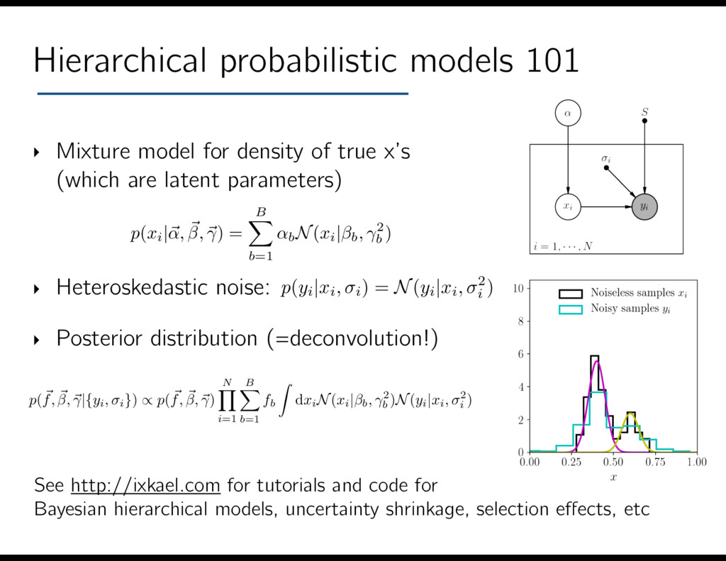
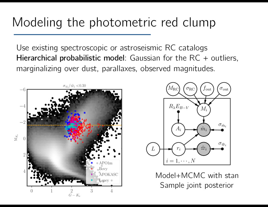
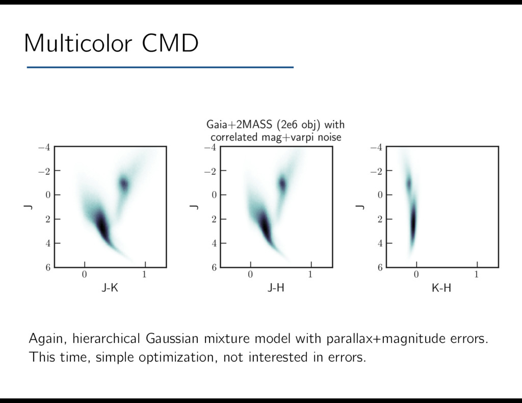
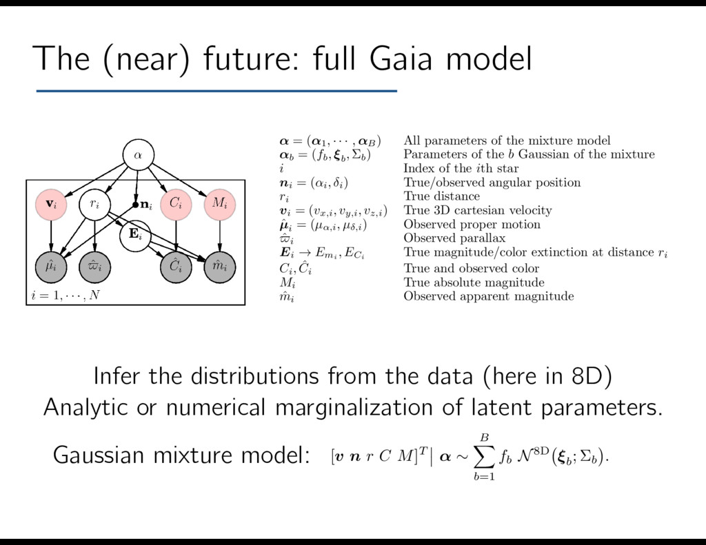
note describing a model of the positions, velocities, proper motions, and colors of stars. If the likelihood function of those is a multivariate Gaussian (which is the case for Gaia, with strong correlations between parallaxes and proper motions), one can adopte a Gaussian Mixture model for their distributions (joint or split) and analytically marginalize over the true velocity, and colors of each star. As a result, one only need to sample the parameters of the mixture model, as well as the distance and extinction of each star. The e↵ective likelihood function is a simple multivariate Gaussian, derived below. This opens the possibility to implement this model in fast inference/modelling languages like Tensorflow, Stan, or Edward. A summary of the notation is provided in the table below. Apologies if there are typos in the text or equations! ↵ = (↵1, · · · , ↵B ) All parameters of the mixture model ↵b = (fb, ⇠b , ⌃b ) Parameters of the b Gaussian of the mixture i Index of the ith star ni = (↵i, i ) True/observed angular position ri True distance vi = (vx,i, vy,i, vz,i ) True 3D cartesian velocity ˆ µi = (µ↵,i, µ ,i ) Observed proper motion ˆ $i Observed parallax Ei ! Emi , ECi True magnitude/color extinction at distance ri Ci, ˆ Ci True and observed color Mi True absolute magnitude ˆ mi Observed apparent magnitude 1 Model Our population/distribution model in 8-dimensional space (3D positions and velocities, plus 2D color–magnitude diagram) is a Gaussian mixture, [v n r C M]T ↵ ⇠ B X b=1 fb N8D ⇠b ; ⌃b . (1) The priors will be specified later. Typically, one would adopt conjugate priors which greatly simply the inference, i.e. a Dirichlet prior on the amplitudes {fb }, and multivariate Gaussian for each mean ⇠b , and Wishard for the covariance ⌃b . The full 5-dimensional likelihood, accounting for any covariance between the measurements, is [ˆ µ↵,i ˆ µ ,i ˆ $i ˆ Ci ˆ mi ]T vi, ni, ri, Ei, Ci, Mi ⇠ N5D ⇣ i ; i ⌘ (2) with the model vector 2 3 and proper motions), one can adopte a Gaussian Mixture model for their distributions (joint marginalize over the true velocity, and colors of each star. As a result, one only need to sam mixture model, as well as the distance and extinction of each star. The e↵ective likelihood funct Gaussian, derived below. This opens the possibility to implement this model in fast inference Tensorflow, Stan, or Edward. A summary of the notation is provided in the table below. Apologies if there are typos in t ↵ = (↵1, · · · , ↵B ) All parameters of the mix ↵b = (fb, ⇠b , ⌃b ) Parameters of the b Gauss i Index of the ith star ni = (↵i, i ) True/observed angular po ri True distance vi = (vx,i, vy,i, vz,i ) True 3D cartesian velocity ˆ µi = (µ↵,i, µ ,i ) Observed proper motion ˆ $i Observed parallax Ei ! Emi , ECi True magnitude/color ext Ci, ˆ Ci True and observed color Mi True absolute magnitude ˆ mi Observed apparent magni 1 Model Our population/distribution model in 8-dimensional space (3D positions and velocities, plus 2D is a Gaussian mixture, [v n r C M]T ↵ ⇠ B X b=1 fb N8D ⇠b ; ⌃b . The priors will be specified later. Typically, one would adopt conjugate priors which greatly s Dirichlet prior on the amplitudes {fb }, and multivariate Gaussian for each mean ⇠b , and Wish The full 5-dimensional likelihood, accounting for any covariance between the measurements Gaussian mixture model: Infer the distributions from the data (here in 8D) Analytic or numerical marginalization of latent parameters.
data-driven models for fully exploiting all of the data without external models. Gaia DR1: high-precision color-magnitude diagrams improved stellar distances binary/triple sequences red-clump calibration Gaia DR2 (April 2018): 3D reconstruction of stellar density, dust, and velocities.