NDGIS 2013 - How to Remain Relevant in the Age of Change or What GIS Pros Can Do to Keep their Skills in Demand

Transcript

1. How to Remain Relevant in the Age of Change James Fee Founder – Spatially Adjusted or What GIS Pros Can Do to Keep their Skills in Demand
2. What is GIS?
3. What is GIS? Who Cares?
4. What are GIS Professionals?
5. What are GIS Professionals? Programmers!
6. Say
 Wut?
7. Programmer 
 /= 
 Developer Photo by Joachim S. Müller - http://flic.kr/p/egrei2
10. James’ Definition of a GIS Professional Someone digitally creates and "manipulates" spatial areas that may be jurisdictional, purpose, or application-oriented.
11. attribution: ESRI International User Conference - 2011 - San Diego, California by Kris Krüg http://flic.kr/p/a2rdhq CC BY-NC-SA 2.0
12. Embrace the Tools of Programmers
14. GIS
15. Esri in the 70’s
16. ArcInfo
17. ARC/INFO Required Prime Computer
25. ArcGIS Desktop
26. ArcGIS Desktop
27. ArcGIS Desktop
31. Why The History Lesson?
32. Photo by dullhunk - http://flic.kr/p/zDLZm
34. A Simpler Time
35. A Simpler Time
36. 
 Problems with Wizards • Wizards cause us to conform • Options are either preset or confusing • Lack of documenting the process
37. Familiarity is a Tough Nut to Crack Most GIS Professionals only know ArcToolbox
41. With the Command Line • Freedom to work with the data as you want • Better understanding of the commands • Combined with scripting you have a recipe for future work. AKA documentation!
42. Programming GIS 1999-2004
43. Programming GIS 1999-2004 • Start up ArcCatalog (wait 2-4 min while it loads)
44. Programming GIS 1999-2004 • Start up ArcCatalog (wait 2-4 min while it loads) • Browse for toolbox (clicking through the endless tree)
45. Programming GIS 1999-2004 • Start up ArcCatalog (wait 2-4 min while it loads) • Browse for toolbox (clicking through the endless tree) • Open tool dialog
46. Programming GIS 1999-2004 • Start up ArcCatalog (wait 2-4 min while it loads) • Browse for toolbox (clicking through the endless tree) • Open tool dialog • Browse for input dataset
47. Programming GIS 1999-2004 • Start up ArcCatalog (wait 2-4 min while it loads) • Browse for toolbox (clicking through the endless tree) • Open tool dialog • Browse for input dataset • Browse for any optional data for analysis
48. Programming GIS 1999-2004 • Start up ArcCatalog (wait 2-4 min while it loads) • Browse for toolbox (clicking through the endless tree) • Open tool dialog • Browse for input dataset • Browse for any optional data for analysis • Browse for an output location
49. Programming GIS 1999-2004 • Start up ArcCatalog (wait 2-4 min while it loads) • Browse for toolbox (clicking through the endless tree) • Open tool dialog • Browse for input dataset • Browse for any optional data for analysis • Browse for an output location • Fill out options
50. Programming GIS 1999-2004 • Start up ArcCatalog (wait 2-4 min while it loads) • Browse for toolbox (clicking through the endless tree) • Open tool dialog • Browse for input dataset • Browse for any optional data for analysis • Browse for an output location • Fill out options • Click OK and pray it doesn’t crash
51. Programming GIS the ArcINFO Way
52. Programming GIS the ArcINFO Way • Start up Command Prompt (about a second)
53. Programming GIS the ArcINFO Way • Start up Command Prompt (about a second) • Type simple command (BUILD, CLIP, etc)
54. Programming GIS the ArcINFO Way • Start up Command Prompt (about a second) • Type simple command (BUILD, CLIP, etc) • Hit Enter
55. Programming GIS the ArcINFO Way • Start up Command Prompt (about a second) • Type simple command (BUILD, CLIP, etc) • Hit Enter • Tell everyone how hard it was
56. AML Scripting
 in ARC/INFO clip soils studbndy stdysoil
57. Where is Python Used?
58. Where is Python Used? • GIS Applications (ArcGIS, QGIS, Safe FME, Autodesk)
59. Where is Python Used? • GIS Applications (ArcGIS, QGIS, Safe FME, Autodesk) • Web Frameworks (WeoGeo.com, Google)
60. Where is Python Used? • GIS Applications (ArcGIS, QGIS, Safe FME, Autodesk) • Web Frameworks (WeoGeo.com, Google) • Anywhere (Corel, Civilization, Gmail)
61. Where is Python Used? • GIS Applications (ArcGIS, QGIS, Safe FME, Autodesk) • Web Frameworks (WeoGeo.com, Google) • Anywhere (Corel, Civilization, Gmail) • Become the de-facto scripting language
62. ArcPy, the New Command Line
63. ArcPy, the New Command Line • Much like the Arc prompt and AML, ArcPy and Python give us a powerful analysis and scripting method.
64. ArcPy, the New Command Line • Much like the Arc prompt and AML, ArcPy and Python give us a powerful analysis and scripting method. • ArcPy builds on the commands we learned 15 years ago.
65. ArcPy, the New Command Line • Much like the Arc prompt and AML, ArcPy and Python give us a powerful analysis and scripting method. • ArcPy builds on the commands we learned 15 years ago. • ArcPy is integrated in ArcMap
66. ArcPy, the New Command Line • Much like the Arc prompt and AML, ArcPy and Python give us a powerful analysis and scripting method. • ArcPy builds on the commands we learned 15 years ago. • ArcPy is integrated in ArcMap • Python can be extended to other GIS platforms such as QGIS.
67. Python Scripting
 in ArcGIS arcpy.Clip_analysis(soils.shp, studbndy.shp, stdysoil) clip soils studbndy stdysoil
68. Python Scripting With ArcPy import  arcpy   from  arcpy  import  env   env.workspace  =  "c:/workspace"   #  variables
 in_features  =  "soils.shp"   clip_features  =  "study_boundary.shp"   out_feature_class  =  "c:/workspace/output/study_area_soils.shp"   xy_tolerance  =  ""   #  Execute  Clip   arcpy.Clip_analysis(in_features,  clip_features,
 out_feature_class,  xy_tolerance)
69. Python Scripting With ArcPy import  arcpy   from  arcpy  import  env   env.workspace  =  "c:/workspace"   #  variables
 in_features  =  "soils.shp"   clip_features  =  "study_boundary.shp"   out_feature_class  =  "c:/workspace/output/study_area_soils.shp"   xy_tolerance  =  ""   #  Execute  Clip   arcpy.Clip_analysis(in_features,  clip_features,
 out_feature_class,  xy_tolerance)
70. http://www.flickr.com/photos/wwarby/2989238425/ Python
71. Export to KML import  arcpy   arcpy.CheckOutExtension(“3D”)   env.workspace  =  "c:/workspace"   #  variables
 in_feature  =  "c:/data/TIGER2009/04/ARIZONA/tl_2009_04_county.lyr"   out_feature  =  "c:/temp/output.kmz"   #  Execute  KML  Export   arcpy.LayerToKML_conversion(in_feature,  out_feature,1)
72. Export to KML arcpy.LayerToKML_conversion(input.shp, output.kml, scale)
73. Python Libraries
77. If you like GIS, you like statistics
78. If you like GIS, you like statistics If you like statistics, you like baseball
79. If you like GIS, you like statistics If you like statistics, you like baseball If you like baseball, you should root for the 2010 and 2012 World Series Champion San Francisco Giants
80. Baseball as an Excuse to Program
82. NYY 95 67 .586 +136 BAL 93 69 .574 +7 TAM 90 72 .556 +120 TOR 73 89 .451 -68 BOS 69 93 .426 -72 DET 88 74 .543 +56 CHS 85 77 .525 +72 KAN 72 90 .444 -70 CLE 68 94 .420 -178 MIN 66 96 .407 -131 OAK 94 68 .580 +99 TEX 93 69 .574 +101 LAA 89 73 .549 +68 SEA 75 87 .463 -32 WAS 98 64 .605 +137 ATL 94 68 .580 +100 PHI 81 81 .500 +4 NYM 74 88 .457 -59 MIA 69 93 .426 -115 CIN 97 65 .599 +81 STL 88 74 .543 +117 MIL 83 79 .512 +43 PIT 79 83 .488 -23 CHC 61 101 .377 -146 HOU 55 107 .340 -211 SFG 94 68 .580 +69 LAD 86 76 .531 +40 ARI 81 81 .500 +46 SDP 76 86 .469 -59 COL 64 98 .395 -132
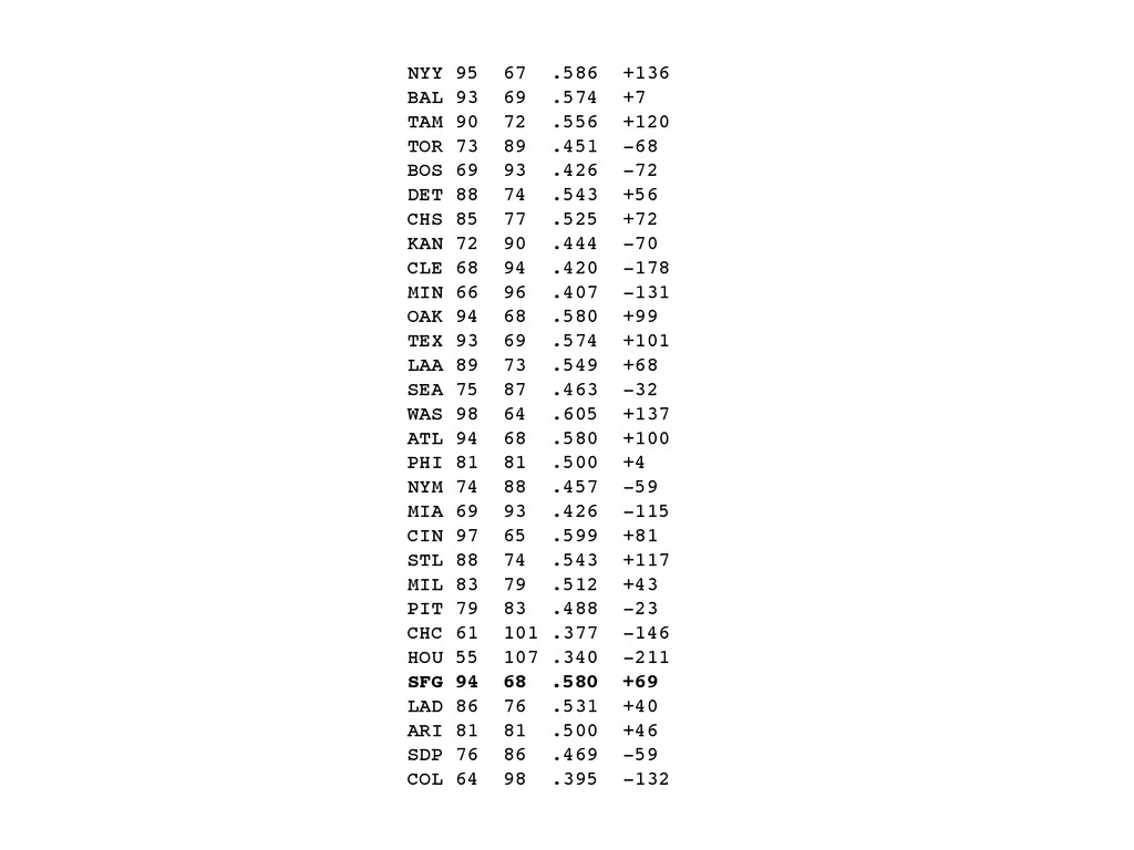
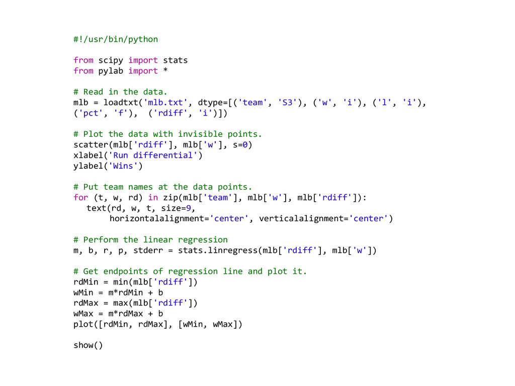
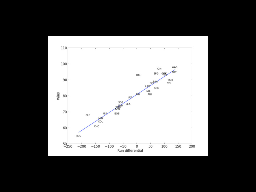
84. #!/usr/bin/python   from  scipy  import  stats   from  pylab  import  *   #  Read  in  the  data.   mlb  =  loadtxt('mlb.txt',  dtype=[('team',  'S3'),  ('w',  'i'),  ('l',  'i'),   ('pct',  'f'),    ('rdiff',  'i')])   #  Plot  the  data  with  invisible  points.   scatter(mlb['rdiff'],  mlb['w'],  s=0)   xlabel('Run  differential')   ylabel('Wins')   #  Put  team  names  at  the  data  points.   for  (t,  w,  rd)  in  zip(mlb['team'],  mlb['w'],  mlb['rdiff']):     text(rd,  w,  t,  size=9,           horizontalalignment='center',  verticalalignment='center')               #  Perform  the  linear  regression   m,  b,  r,  p,  stderr  =  stats.linregress(mlb['rdiff'],  mlb['w'])   #  Get  endpoints  of  regression  line  and  plot  it.   rdMin  =  min(mlb['rdiff'])   wMin  =  m*rdMin  +  b   rdMax  =  max(mlb['rdiff'])   wMax  =  m*rdMax  +  b   plot([rdMin,  rdMax],  [wMin,  wMax])   show()
87. Rainbows and Unicorns
88. PySAL https://geodacenter.asu.edu/pysal
89. OpenGeoDa • Spatial Data Manipulation • Visualization and Queries • Mapping • Exploratory Data Analysis • Spatial Statistics https://geodacenter.asu.edu/
91. The Future for GIS Professionals
92. So You Want to be a
 Word Processor
93. The Future for
 Word Processors
95. If You... • Put points on a map and throw up a scale bar • Perform geoprocessing without Python or Model Builder • Have a job description of “Plotter Operator” • Have no idea what “fuzzy tolerance” is
96. You’ll be out of a job
97. If You... • Embrace Python as your GIS tool of choice. • Use Model Builder to automate your work flows. • Learn new tools such as TileMill/Mapnik/ PostGIS
99. History of GIS Professionals Photo by Johnson Cameraface - http://flic.kr/p/dwQdSq
102. Rise of the Database
103. Rise of the Web
111. GIS
112. GIS Professionals Assimilate New Technology
113. Technology Comes Early to GIS
114. Don’t Settle Down with GIS
115. Cutting edge is lots of work.
117. Thanks! James Fee james@spatiallyadjusted.net @cageyjames spatiallyadjusted.com
118. Thanks! James Fee james@spatiallyadjusted.net @cageyjames spatiallyadjusted.com