Prony, LP or Super-Resolution for Sparse Interpolation?

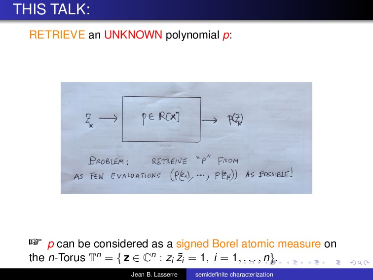
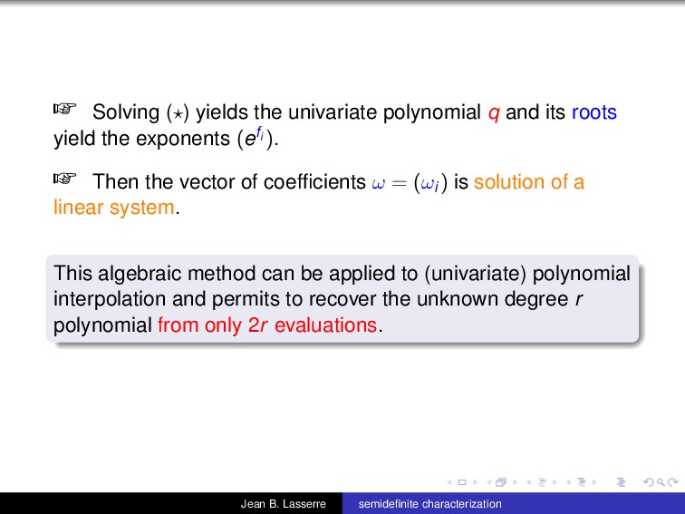
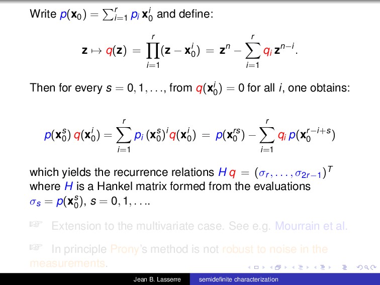
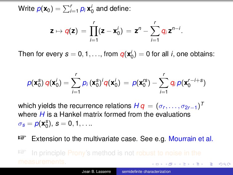
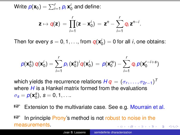
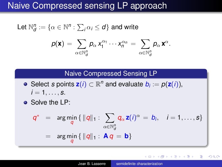
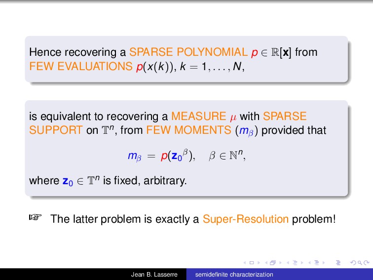
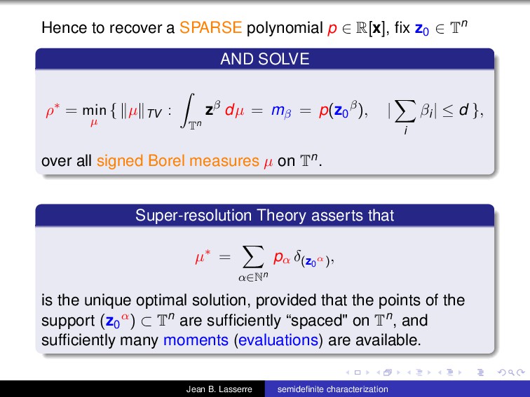
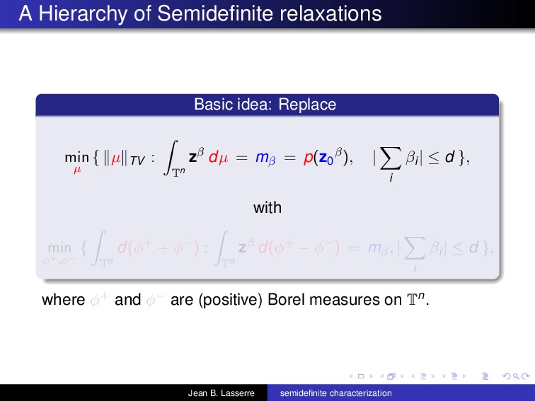
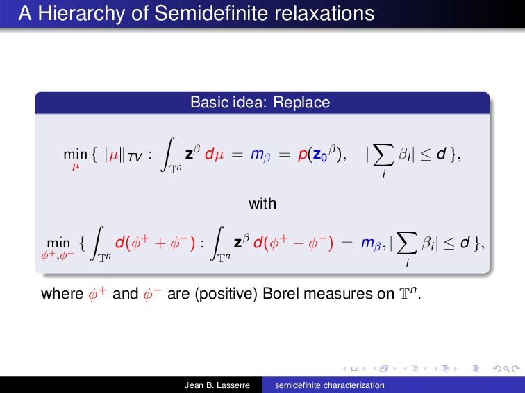
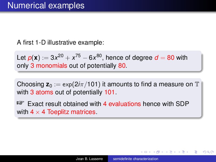
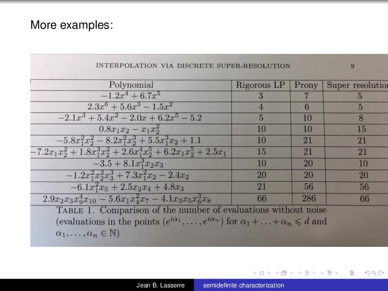
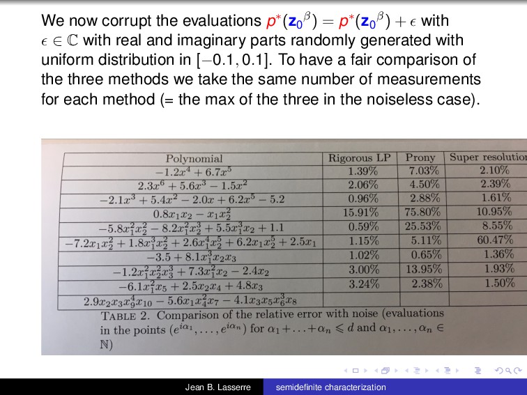
We describe how sparse interpolation of polynomials can be viewed as a specific "discrete" super-resolution problem that can be solved efficiently by using the Moment-SOS hierarchy. It is also compared with an equivalent LP-approach with L1 sparsity inducing norm, as well as the algebraic Prony's method.

Transcript

1. . . . . . . . . . . . . . . . . . . . . . . . . . . . . . . . . . . . . . . . . Prony, LP or Super-Resolution for Sparse Interpolation? Jean B. Lasserre LAAS-CNRS and Institute of Mathematics, Toulouse, France Simons Institute, UC Berkeley, November 2017 ⋆ Research funded by the European Research Council (ERC) under the European Union’s Horizon 2020 research and innovation program (grant agreement 666981 TAMING) Jean B. Lasserre semidefinite characterization
2. . . . . . . . . . . . . . . . . . . . . . . . . . . . . . . . . . . . . . . . . Research done in collaboration with: Cédric Josz (Post-doc, LAAS-CNRS) Bernard Mourrain (Senior researcher, INRIA) Sparse polynomial interpolation: compressed sensing, super resolution, or Prony? arXiv:1708.06187 Jean B. Lasserre semidefinite characterization
3. . . . . . . . . . . . . . . . . . . . . . . . . . . . . . . . . . . . . . . . . Message When studying some questions, polynomials can be (or, should be (?)) associated with (signed) measures on appropriate geometrical objects. For instance the DUAL CONE P∗ d of Pd = nonnegative homogeneous polynomials of degree 2d on Rn (measures) can be identified with the convex cone of sums of finitely many 2d-powers of LINEAR FORMS (a subset of Pd ) Jean B. Lasserre semidefinite characterization
4. . . . . . . . . . . . . . . . . . . . . . . . . . . . . . . . . . . . . . . . . For instance for 3-tensor completion or 3-tensor decomposition, a symmetric tensor A = (Aijk )1≤i,j,k≤n can be interpreted as MOMENTS of some ATOMIC measure µ on unit sphere Sn−1: A = ∫ Sn−1 x ⊗ x ⊗ x dµ(x), ( → A = ∑ i λi ui ⊗ ui ⊗ ui ) GIVEN A, Recovery of the decomposition of A (or the entire A) by the Moment-SOS approach Tang & Sha (2015), Potechin & Steurer (2017) Jean B. Lasserre semidefinite characterization
5. . . . . . . . . . . . . . . . . . . . . . . . . . . . . . . . . . . . . . . . . THIS TALK: RETRIEVE an UNKNOWN polynomial p: p can be considered as a signed Borel atomic measure on the n-Torus Tn = { z ∈ Cn : zi ¯ zi = 1, i = 1, . . . , n}. Jean B. Lasserre semidefinite characterization
6. . . . . . . . . . . . . . . . . . . . . . . . . . . . . . . . . . . . . . . . . IF p IS A SPARSE POLYNOMIAL ⇓ THEN FEW EVALUATIONS ARE NEEDED Jean B. Lasserre semidefinite characterization
7. . . . . . . . . . . . . . . . . . . . . . . . . . . . . . . . . . . . . . . . . I. PRONY METHOD Originally, Prony’s method considers a signal z → h(x) = r ∑ i=1 ωi efi x ∈ C, x ∈ R and recovers the unknown data (ωi, fi)r i=1 from 2r measurements (σi := h(xi))i=0,...,2r−1 . Consider the polynomial: x → r ∏ i=1 (x − efi ) = xr − r−1 ∑ j=0 qj xj. Its vector of coefficients q = (qj)r−1 j=0 satisfies (⋆) H q = (σr , . . . , σ2r−1)T , with H a Hankel matrix formed from the measurements (σj)2r−2 j=0 . Jean B. Lasserre semidefinite characterization
8. . . . . . . . . . . . . . . . . . . . . . . . . . . . . . . . . . . . . . . . . I. PRONY METHOD Originally, Prony’s method considers a signal z → h(x) = r ∑ i=1 ωi efi x ∈ C, x ∈ R and recovers the unknown data (ωi, fi)r i=1 from 2r measurements (σi := h(xi))i=0,...,2r−1 . Consider the polynomial: x → r ∏ i=1 (x − efi ) = xr − r−1 ∑ j=0 qj xj. Its vector of coefficients q = (qj)r−1 j=0 satisfies (⋆) H q = (σr , . . . , σ2r−1)T , with H a Hankel matrix formed from the measurements (σj)2r−2 j=0 . Jean B. Lasserre semidefinite characterization
9. . . . . . . . . . . . . . . . . . . . . . . . . . . . . . . . . . . . . . . . . Solving (⋆) yields the univariate polynomial q and its roots yield the exponents (efi ). Then the vector of coefficients ω = (ωi) is solution of a linear system. This algebraic method can be applied to (univariate) polynomial interpolation and permits to recover the unknown degree r polynomial from only 2r evaluations. Jean B. Lasserre semidefinite characterization
10. . . . . . . . . . . . . . . . . . . . . . . . . . . . . . . . . . . . . . . . . Solving (⋆) yields the univariate polynomial q and its roots yield the exponents (efi ). Then the vector of coefficients ω = (ωi) is solution of a linear system. This algebraic method can be applied to (univariate) polynomial interpolation and permits to recover the unknown degree r polynomial from only 2r evaluations. Jean B. Lasserre semidefinite characterization
11. . . . . . . . . . . . . . . . . . . . . . . . . . . . . . . . . . . . . . . . . Solving (⋆) yields the univariate polynomial q and its roots yield the exponents (efi ). Then the vector of coefficients ω = (ωi) is solution of a linear system. This algebraic method can be applied to (univariate) polynomial interpolation and permits to recover the unknown degree r polynomial from only 2r evaluations. Jean B. Lasserre semidefinite characterization
12. . . . . . . . . . . . . . . . . . . . . . . . . . . . . . . . . . . . . . . . . Write p(x0) = ∑ r i=1 pi xi 0 and define: z → q(z) = r ∏ i=1 (z − xi 0 ) = zn − r ∑ i=1 qi zn−i. Then for every s = 0, 1, . . ., from q(xi 0 ) = 0 for all i, one obtains: p(xs 0 ) q(xi 0 ) = r ∑ i=1 pi (xs 0 )iq(xi 0 ) = p(xrs 0 ) − r ∑ i=1 qi p(xr−i+s 0 ) which yields the recurrence relations H q = (σr , . . . , σ2r−1)T where H is a Hankel matrix formed from the evaluations σs = p(xs 0 ), s = 0, 1, . . .. Extension to the multivariate case. See e.g. Mourrain et al. In principle Prony’s method is not robust to noise in the measurements. Jean B. Lasserre semidefinite characterization
13. . . . . . . . . . . . . . . . . . . . . . . . . . . . . . . . . . . . . . . . . Write p(x0) = ∑ r i=1 pi xi 0 and define: z → q(z) = r ∏ i=1 (z − xi 0 ) = zn − r ∑ i=1 qi zn−i. Then for every s = 0, 1, . . ., from q(xi 0 ) = 0 for all i, one obtains: p(xs 0 ) q(xi 0 ) = r ∑ i=1 pi (xs 0 )iq(xi 0 ) = p(xrs 0 ) − r ∑ i=1 qi p(xr−i+s 0 ) which yields the recurrence relations H q = (σr , . . . , σ2r−1)T where H is a Hankel matrix formed from the evaluations σs = p(xs 0 ), s = 0, 1, . . .. Extension to the multivariate case. See e.g. Mourrain et al. In principle Prony’s method is not robust to noise in the measurements. Jean B. Lasserre semidefinite characterization
14. . . . . . . . . . . . . . . . . . . . . . . . . . . . . . . . . . . . . . . . . Write p(x0) = ∑ r i=1 pi xi 0 and define: z → q(z) = r ∏ i=1 (z − xi 0 ) = zn − r ∑ i=1 qi zn−i. Then for every s = 0, 1, . . ., from q(xi 0 ) = 0 for all i, one obtains: p(xs 0 ) q(xi 0 ) = r ∑ i=1 pi (xs 0 )iq(xi 0 ) = p(xrs 0 ) − r ∑ i=1 qi p(xr−i+s 0 ) which yields the recurrence relations H q = (σr , . . . , σ2r−1)T where H is a Hankel matrix formed from the evaluations σs = p(xs 0 ), s = 0, 1, . . .. Extension to the multivariate case. See e.g. Mourrain et al. In principle Prony’s method is not robust to noise in the measurements. Jean B. Lasserre semidefinite characterization
15. . . . . . . . . . . . . . . . . . . . . . . . . . . . . . . . . . . . . . . . . Naive Compressed sensing LP approach Let Nn d := {α ∈ Nn : ∑ i αi ≤ d} and write p(x) = ∑ α∈Nn d pα xα1 1 · · · xαn n = ∑ α∈Nn d pα xα. Naive Compressed Sensing LP Select s points z(i) ⊂ Rn and evaluate bi := p(z(i)), i = 1, . . . , s. Solve the LP: q∗ = arg min q { ∥q∥1 : ∑ α∈Nn d qα z(i)α = bi, i = 1, . . . , s} = arg min q { ∥q∥1 : A q = b} Jean B. Lasserre semidefinite characterization
16. . . . . . . . . . . . . . . . . . . . . . . . . . . . . . . . . . . . . . . . . central idea The unknown vector q of this LP has potentially high dimension ( n+d n ) and the sparsity-inducing norm ∥ · ∥1 aims at finding a SPARSE solution q∗, that is, a vector with few non-zero entries. The pseudo-norm x → ∥x∥0 := #{i : xi ̸= 0} counts the number of non-zero entries of a vector x. Compressed sensing theory asserts that if the constraint-matrix A ∈ Rm×n satisfies the Restricted Isometry Property (RIP) then solving min { ∥x∥1 : A x = b} permits to recover an optimal solution to the non-convex problem min { ∥x∥0 : A x = b} provided that m is sufficiently large (but not too large). Jean B. Lasserre semidefinite characterization
17. . . . . . . . . . . . . . . . . . . . . . . . . . . . . . . . . . . . . . . . . central idea The unknown vector q of this LP has potentially high dimension ( n+d n ) and the sparsity-inducing norm ∥ · ∥1 aims at finding a SPARSE solution q∗, that is, a vector with few non-zero entries. The pseudo-norm x → ∥x∥0 := #{i : xi ̸= 0} counts the number of non-zero entries of a vector x. Compressed sensing theory asserts that if the constraint-matrix A ∈ Rm×n satisfies the Restricted Isometry Property (RIP) then solving min { ∥x∥1 : A x = b} permits to recover an optimal solution to the non-convex problem min { ∥x∥0 : A x = b} provided that m is sufficiently large (but not too large). Jean B. Lasserre semidefinite characterization
18. . . . . . . . . . . . . . . . . . . . . . . . . . . . . . . . . . . . . . . . . However, in our setting of the Naive LP for Sparse Interpolation, the associated matrix A DOES NOT SATISFY the RIP property! ⇓ There is no guarantee to recover the sparse polynomial p by solving the associated NAIVE Compressed Sensing LP Jean B. Lasserre semidefinite characterization
19. . . . . . . . . . . . . . . . . . . . . . . . . . . . . . . . . . . . . . . . . However, in our setting of the Naive LP for Sparse Interpolation, the associated matrix A DOES NOT SATISFY the RIP property! ⇓ There is no guarantee to recover the sparse polynomial p by solving the associated NAIVE Compressed Sensing LP Jean B. Lasserre semidefinite characterization
20. . . . . . . . . . . . . . . . . . . . . . . . . . . . . . . . . . . . . . . . . Super-Resolution Let Tn = {z ∈ Cn : zi ¯ zi = 1, i = 1, . . . , n}. Given a signed Borel measure µ∗ = N ∑ k=1 θk δz(k) , z(k) ∈ Tn, with FINITE SUPPORT on the torus Tn, and given all moments mα := ∫ Tn zα dµ(z), | n ∑ i=1 αi| ≤ d, UP TO DEGREE d, can we recover the support (z(1), . . . , z(N)) AND the weights (θ1, . . . , θN)? Jean B. Lasserre semidefinite characterization
21. . . . . . . . . . . . . . . . . . . . . . . . . . . . . . . . . . . . . . . . . Super-Resolution Let Tn = {z ∈ Cn : zi ¯ zi = 1, i = 1, . . . , n}. Given a signed Borel measure µ∗ = N ∑ k=1 θk δz(k) , z(k) ∈ Tn, with FINITE SUPPORT on the torus Tn, and given all moments mα := ∫ Tn zα dµ(z), | n ∑ i=1 αi| ≤ d, UP TO DEGREE d, can we recover the support (z(1), . . . , z(N)) AND the weights (θ1, . . . , θN)? Jean B. Lasserre semidefinite characterization
22. . . . . . . . . . . . . . . . . . . . . . . . . . . . . . . . . . . . . . . . . SUPER-RESOLUTION Theory asserts that: I. µ∗ is the unique optimal solution of the optimization problem min { ∥µ∥TV : ∫ Tn zα dµ = mα, | ∑ i αi| ≤ d }, over all signed Borel measures µ on Tn, .... provided that d is sufficiently large and the points (z(k)) are sufficiently “geometrically separated". II. If n = 1 then the atoms are obtained from solving a SINGLE SDP. Candès & Fernandez-Granda, Comm. Pure & Appl. Math. (2013) Extension to the multivariate case: de Castro et al., IEEE Trans. Info. Theory (2017) Jean B. Lasserre semidefinite characterization
23. . . . . . . . . . . . . . . . . . . . . . . . . . . . . . . . . . . . . . . . . SUPER-RESOLUTION Theory asserts that: I. µ∗ is the unique optimal solution of the optimization problem min { ∥µ∥TV : ∫ Tn zα dµ = mα, | ∑ i αi| ≤ d }, over all signed Borel measures µ on Tn, .... provided that d is sufficiently large and the points (z(k)) are sufficiently “geometrically separated". II. If n = 1 then the atoms are obtained from solving a SINGLE SDP. Candès & Fernandez-Granda, Comm. Pure & Appl. Math. (2013) Extension to the multivariate case: de Castro et al., IEEE Trans. Info. Theory (2017) Jean B. Lasserre semidefinite characterization
24. . . . . . . . . . . . . . . . . . . . . . . . . . . . . . . . . . . . . . . . . PRONY METHOD can also be used to recover µ∗ and requires knowledge of less “moments" than Super-Resolution. For instance in the univariate case PRONY requires 2N moments while Super-Resolution requires 4N moments. However it is argued that Super-Resolution is more robust to noise in the data (mα ). Jean B. Lasserre semidefinite characterization
25. . . . . . . . . . . . . . . . . . . . . . . . . . . . . . . . . . . . . . . . . Back to sparse interpolation A crucial observation: Let z0 ∈ Tn be fixed and p ∈ R[x]d . Then for each β ∈ Nn: p(z0 β) = ∑ α∈Nn d pα (z0 β)α = ∑ α∈Nn d pα (z0 α)β = ∑ α∈Nn d pα ⟨zβ, δ(z0 α) ⟩ = ⟨ zβ, ∑ α∈Nn d pα δ(z0 α) µ ⟩ = ∫ Tn zβ dµ Jean B. Lasserre semidefinite characterization
26. . . . . . . . . . . . . . . . . . . . . . . . . . . . . . . . . . . . . . . . . Therefore ... given an arbitrary fixed z0 ∈ Tn (i) Every polynomial x → ∑ α pα xα can be viewed as a SIGNED BOREL MEASURE µ on Tn: - WITH FINITE SUPPORT (z0 α)α∈Nn ⊂ Tn, - AND WEIGHTS (pα)α∈Nn ⊂ R. (ii) The evaluation p(z0 β) is the MOMENT ∫ Tn zβ dµ, with β ∈ Nn. Jean B. Lasserre semidefinite characterization
27. . . . . . . . . . . . . . . . . . . . . . . . . . . . . . . . . . . . . . . . . Hence recovering a SPARSE POLYNOMIAL p ∈ R[x] from FEW EVALUATIONS p(x(k)), k = 1, . . . , N, is equivalent to recovering a MEASURE µ with SPARSE SUPPORT on Tn, from FEW MOMENTS (mβ) provided that mβ = p(z0 β), β ∈ Nn, where z0 ∈ Tn is fixed, arbitrary. The latter problem is exactly a Super-Resolution problem! Jean B. Lasserre semidefinite characterization
28. . . . . . . . . . . . . . . . . . . . . . . . . . . . . . . . . . . . . . . . . Hence to recover a SPARSE polynomial p ∈ R[x], fix z0 ∈ Tn AND SOLVE ρ∗ = min µ { ∥µ∥TV : ∫ Tn zβ dµ = mβ = p(z0 β), | ∑ i βi| ≤ d }, over all signed Borel measures µ on Tn. Super-resolution Theory asserts that µ∗ = ∑ α∈Nn pα δ(z0 α) , is the unique optimal solution, provided that the points of the support (z0 α) ⊂ Tn are sufficiently “spaced" on Tn, and sufficiently many moments (evaluations) are available. Jean B. Lasserre semidefinite characterization
29. . . . . . . . . . . . . . . . . . . . . . . . . . . . . . . . . . . . . . . . . A Hierarchy of Semidefinite relaxations Basic idea: Replace min µ { ∥µ∥TV : ∫ Tn zβ dµ = mβ = p(z0 β), | ∑ i βi| ≤ d }, with min ϕ+,ϕ− { ∫ Tn d(ϕ+ + ϕ−) : ∫ Tn zβ d(ϕ+ − ϕ−) = mβ, | ∑ i βi| ≤ d }, where ϕ+ and ϕ− are (positive) Borel measures on Tn. Jean B. Lasserre semidefinite characterization
30. . . . . . . . . . . . . . . . . . . . . . . . . . . . . . . . . . . . . . . . . A Hierarchy of Semidefinite relaxations Basic idea: Replace min µ { ∥µ∥TV : ∫ Tn zβ dµ = mβ = p(z0 β), | ∑ i βi| ≤ d }, with min ϕ+,ϕ− { ∫ Tn d(ϕ+ + ϕ−) : ∫ Tn zβ d(ϕ+ − ϕ−) = mβ, | ∑ i βi| ≤ d }, where ϕ+ and ϕ− are (positive) Borel measures on Tn. Jean B. Lasserre semidefinite characterization
31. . . . . . . . . . . . . . . . . . . . . . . . . . . . . . . . . . . . . . . . . Then solve the hierarchy of semidefinite relaxations ρs = min (ϕ+ β ),(ϕ− β ) { ϕ+ 0 + ϕ− 0 : s.t. ϕ+ β − ϕ− β = mβ, | ∑ i βi| ≤ d Ts(ϕ+), Ts(ϕ−) ⪰ 0} for all s with 2s ≥ d. where Ts(ϕ+) (resp. Ts(ϕ−)) are the respective multivariate Toeplitz moment matrices of ϕ+ and ϕ− on the torus Tn. In dimensions n = 1, 2 ρs = ρ∗ for some s ∈ N, and lim s→∞ ρs = ρ∗ in general. In practice CONVERGENCE IS FINITE and and extraction procedure for the support and the weights is available. Jean B. Lasserre semidefinite characterization
32. . . . . . . . . . . . . . . . . . . . . . . . . . . . . . . . . . . . . . . . . Then solve the hierarchy of semidefinite relaxations ρs = min (ϕ+ β ),(ϕ− β ) { ϕ+ 0 + ϕ− 0 : s.t. ϕ+ β − ϕ− β = mβ, | ∑ i βi| ≤ d Ts(ϕ+), Ts(ϕ−) ⪰ 0} for all s with 2s ≥ d. where Ts(ϕ+) (resp. Ts(ϕ−)) are the respective multivariate Toeplitz moment matrices of ϕ+ and ϕ− on the torus Tn. In dimensions n = 1, 2 ρs = ρ∗ for some s ∈ N, and lim s→∞ ρs = ρ∗ in general. In practice CONVERGENCE IS FINITE and and extraction procedure for the support and the weights is available. Jean B. Lasserre semidefinite characterization
33. . . . . . . . . . . . . . . . . . . . . . . . . . . . . . . . . . . . . . . . . Then solve the hierarchy of semidefinite relaxations ρs = min (ϕ+ β ),(ϕ− β ) { ϕ+ 0 + ϕ− 0 : s.t. ϕ+ β − ϕ− β = mβ, | ∑ i βi| ≤ d Ts(ϕ+), Ts(ϕ−) ⪰ 0} for all s with 2s ≥ d. where Ts(ϕ+) (resp. Ts(ϕ−)) are the respective multivariate Toeplitz moment matrices of ϕ+ and ϕ− on the torus Tn. In dimensions n = 1, 2 ρs = ρ∗ for some s ∈ N, and lim s→∞ ρs = ρ∗ in general. In practice CONVERGENCE IS FINITE and and extraction procedure for the support and the weights is available. Jean B. Lasserre semidefinite characterization
34. . . . . . . . . . . . . . . . . . . . . . . . . . . . . . . . . . . . . . . . . Rigorous Compressed sensing LP • In the interpolation context one may choose z0 := (e2i π/N, . . . , e2i π/N) ∈ Tn for sufficiently large N. • Then the unknown sparse Borel measure µ on Tn (equivalently the unknown sparse polynomial p ∈ R[x]) is supported on the fixed grid (e2iπk/N)k=0,1,...,N)n. • That is: the Super-Resolution problem becomes a DISCRETE SUPER-RESOLUTION problem. Jean B. Lasserre semidefinite characterization
35. . . . . . . . . . . . . . . . . . . . . . . . . . . . . . . . . . . . . . . . . Rigorous Compressed sensing LP • In the interpolation context one may choose z0 := (e2i π/N, . . . , e2i π/N) ∈ Tn for sufficiently large N. • Then the unknown sparse Borel measure µ on Tn (equivalently the unknown sparse polynomial p ∈ R[x]) is supported on the fixed grid (e2iπk/N)k=0,1,...,N)n. • That is: the Super-Resolution problem becomes a DISCRETE SUPER-RESOLUTION problem. Jean B. Lasserre semidefinite characterization
36. . . . . . . . . . . . . . . . . . . . . . . . . . . . . . . . . . . . . . . . . Rigorous Compressed sensing LP • In the interpolation context one may choose z0 := (e2i π/N, . . . , e2i π/N) ∈ Tn for sufficiently large N. • Then the unknown sparse Borel measure µ on Tn (equivalently the unknown sparse polynomial p ∈ R[x]) is supported on the fixed grid (e2iπk/N)k=0,1,...,N)n. • That is: the Super-Resolution problem becomes a DISCRETE SUPER-RESOLUTION problem. Jean B. Lasserre semidefinite characterization
37. . . . . . . . . . . . . . . . . . . . . . . . . . . . . . . . . . . . . . . . . By Super-Resolution Theory The sparse polynomial p ∈ R[x] is the unique optimal solution of the (Compressed sensing) LP min p∈R[x]t {∥p∥1 : ∑ α pα ((z0 α)β) = p∗(z0 β), | ∑ i βi| ≤ N} Hint: : ∥p∥1 = ∑ α |pα| = ∥µ∥TV . Provides a nice example where exact recovery by compressed sensing is guaranteed even though the RIP is not satisfied. Jean B. Lasserre semidefinite characterization
38. . . . . . . . . . . . . . . . . . . . . . . . . . . . . . . . . . . . . . . . . By Super-Resolution Theory The sparse polynomial p ∈ R[x] is the unique optimal solution of the (Compressed sensing) LP min p∈R[x]t {∥p∥1 : ∑ α pα ((z0 α)β) = p∗(z0 β), | ∑ i βi| ≤ N} Hint: : ∥p∥1 = ∑ α |pα| = ∥µ∥TV . Provides a nice example where exact recovery by compressed sensing is guaranteed even though the RIP is not satisfied. Jean B. Lasserre semidefinite characterization
39. . . . . . . . . . . . . . . . . . . . . . . . . . . . . . . . . . . . . . . . . Numerical examples A first 1-D illustrative example: Let p(x) := 3x20 + x75 − 6x80, hence of degree d = 80 with only 3 monomials out of potentially 80. Choosing z0 := exp(2iπ/101) it amounts to find a measure on T with 3 atoms out of potentially 101. Exact result obtained with 4 evaluations hence with SDP with 4 × 4 Toeplitz matrices. Jean B. Lasserre semidefinite characterization
40. . . . . . . . . . . . . . . . . . . . . . . . . . . . . . . . . . . . . . . . . -1 -0.5 0 0.5 1 Real part -1 -0.5 0 0.5 1 Imaginary part Positive Support in Blue / Negative Support in Red 0 1 2 3 4 5 6 Angle (in radians) -1 -0.8 -0.6 -0.4 -0.2 0 0.2 0.4 0.6 0.8 1 Real part of dual polynomial Interpolation Polynomial Figure: with z0 = exp(2iπ/101) Jean B. Lasserre semidefinite characterization
41. . . . . . . . . . . . . . . . . . . . . . . . . . . . . . . . . . . . . . . . . -1 -0.5 0 0.5 1 Real part -1 -0.5 0 0.5 1 Imaginary part Positive Support in Blue / Negative Support in Red 0 1 2 3 4 5 6 Angle (in radians) -1 -0.8 -0.6 -0.4 -0.2 0 0.2 0.4 0.6 0.8 1 Real part of dual polynomial Interpolation Polynomial Figure: with z0 = exp(i) Jean B. Lasserre semidefinite characterization
42. . . . . . . . . . . . . . . . . . . . . . . . . . . . . . . . . . . . . . . . . More examples: Jean B. Lasserre semidefinite characterization
43. . . . . . . . . . . . . . . . . . . . . . . . . . . . . . . . . . . . . . . . . We now corrupt the evaluations p∗(z0 β) = p∗(z0 β) + ϵ with ϵ ∈ C with real and imaginary parts randomly generated with uniform distribution in [−0.1, 0.1]. To have a fair comparison of the three methods we take the same number of measurements for each method (= the max of the three in the noiseless case). Jean B. Lasserre semidefinite characterization
44. . . . . . . . . . . . . . . . . . . . . . . . . . . . . . . . . . . . . . . . . Preliminary conclusion I. Super-Resolution = Semidefinite Optimization + extraction of atoms from the SDP solution Extraction of atoms is same as PRONY ! But the semidefinite Optimization step helps in the noise case. II. Rigorous LP-compressed sensing behaves well with and without noise but its setup is time-consuming. Jean B. Lasserre semidefinite characterization
45. . . . . . . . . . . . . . . . . . . . . . . . . . . . . . . . . . . . . . . . . Preliminary conclusion I. Super-Resolution = Semidefinite Optimization + extraction of atoms from the SDP solution Extraction of atoms is same as PRONY ! But the semidefinite Optimization step helps in the noise case. II. Rigorous LP-compressed sensing behaves well with and without noise but its setup is time-consuming. Jean B. Lasserre semidefinite characterization
46. . . . . . . . . . . . . . . . . . . . . . . . . . . . . . . . . . . . . . . . . Preliminary conclusion I. Super-Resolution = Semidefinite Optimization + extraction of atoms from the SDP solution Extraction of atoms is same as PRONY ! But the semidefinite Optimization step helps in the noise case. II. Rigorous LP-compressed sensing behaves well with and without noise but its setup is time-consuming. Jean B. Lasserre semidefinite characterization
47. . . . . . . . . . . . . . . . . . . . . . . . . . . . . . . . . . . . . . . . . Thank you! Jean B. Lasserre semidefinite characterization