Increasingly Powerful Tornadoes

Transcript

1. Increasingly Powerful Tornadoes And The Rising Potential for Mass Casualties James B. Elsner (@JBElsner) October 19, 2018 Department of Statistics Florida State University
2. What?
3. How?
5. Where?
6. When? Midnight 2 am 4 am 6 am 8 am 10 am Noon 2 pm 4 pm 6 pm 8 pm 10 pm 0 1000 2000 3000 Time of Day Number of Tornadoes
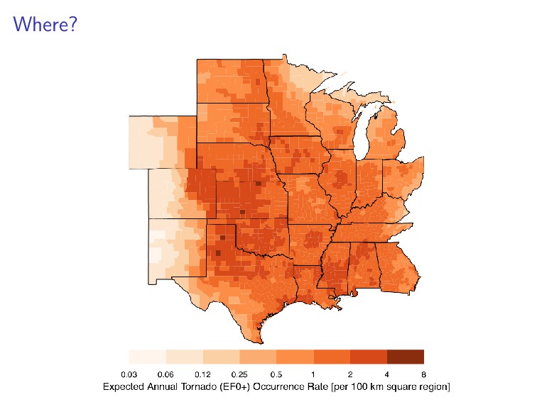
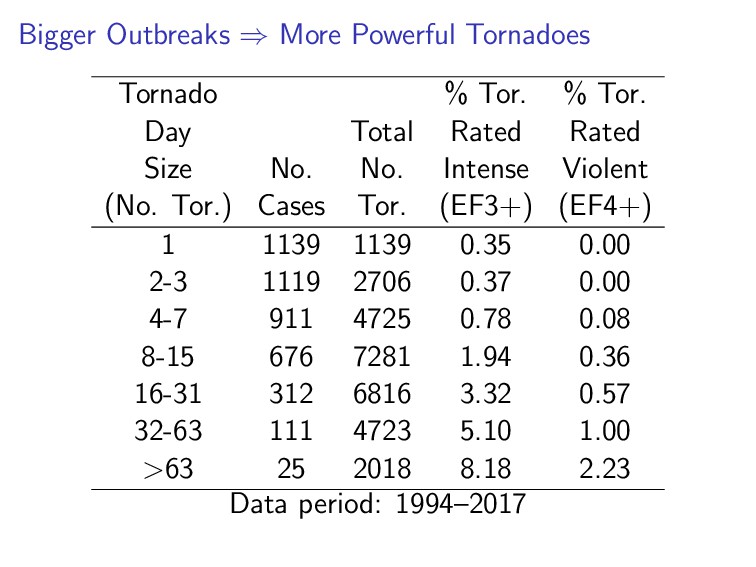
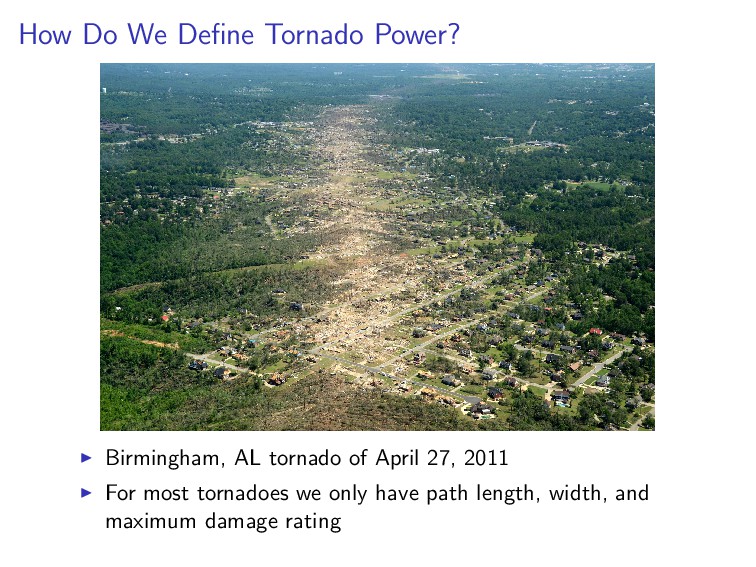
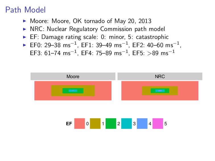
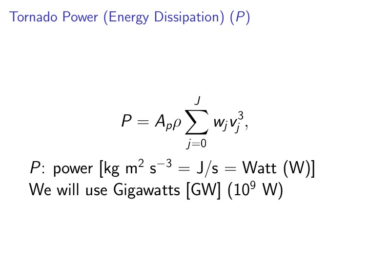
7. Outline of Talk 1. Why Do We Think Tornadoes Are Getting More Powerful? 2. How Do We Define Tornado Power? 3. What Model Do We Use? 4. How Well Does the Model Replicate the Data? 5. What Does the Model Say About the Trend? 6. What Might Be Causing the Trend? 7. Why Is This Important?
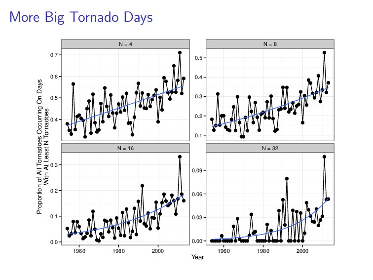
8. More Big Tornado Days N = 4 N = 8 N = 16 N = 32 0.4 0.5 0.6 0.7 0.1 0.2 0.3 0.4 0.5 0.0 0.1 0.2 0.3 0.00 0.03 0.06 0.09 1960 1980 2000 1960 1980 2000 Year Proportion of All Tornadoes Occurring On Days With At Least N Tornadoes
9. Bigger Outbreaks ⇒ More Powerful Tornadoes Tornado % Tor. % Tor. Day Total Rated Rated Size No. No. Intense Violent (No. Tor.) Cases Tor. (EF3+) (EF4+) 1 1139 1139 0.35 0.00 2-3 1119 2706 0.37 0.00 4-7 911 4725 0.78 0.08 8-15 676 7281 1.94 0.36 16-31 312 6816 3.32 0.57 32-63 111 4723 5.10 1.00 >63 25 2018 8.18 2.23 Data period: 1994–2017
10. How Do We Define Tornado Power? Birmingham, AL tornado of April 27, 2011 For most tornadoes we only have path length, width, and maximum damage rating
11. Path Model Moore: Moore, OK tornado of May 20, 2013 NRC: Nuclear Regulatory Commission path model EF: Damage rating scale: 0: minor, 5: catastrophic EF0: 29–38 ms−1, EF1: 39–49 ms−1, EF2: 40–60 ms−1, EF3: 61–74 ms−1, EF4: 75–89 ms−1, EF5: >89 ms−1 Moore NRC EF 0 1 2 3 4 5
12. Tornado Power (Energy Dissipation) (P) P = Ap ρ J j=0 wj v3 j , P: power [kg m2 s−3 = J/s = Watt (W)] We will use Gigawatts [GW] (109 W)
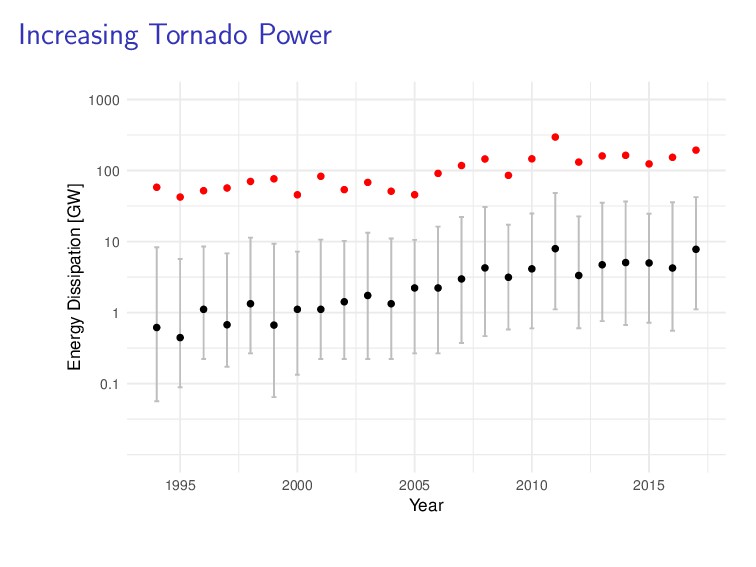
13. Tornado Power By Damage Rating [1994–2017] Energy dissipation (power). Values are in gigawatts (GW) Number of Median Total Mean Power EF Tornadoes Power Power Arithmetic Geometric 0 17906 1 78793 4 1 1 8325 13 408484 49 11 2 2353 94 669704 285 80 3 663 638 872298 1315 507 4 147 1642 522109 3552 1453 5 14 6458 130239 9303 5623
14. Increasing Tornado Power 0.1 1 10 100 1000 1995 2000 2005 2010 2015 Year Energy Dissipation [GW]
15. Variability By Time of Day Midnight 2 am 4 am 6 am 8 am 10 am Noon 2 pm 4 pm 6 pm 8 pm 10 pm 0.0 2.5 5.0 7.5 Time of Day Average (geometric) Tornado Power (GW)
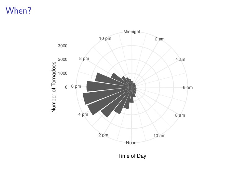
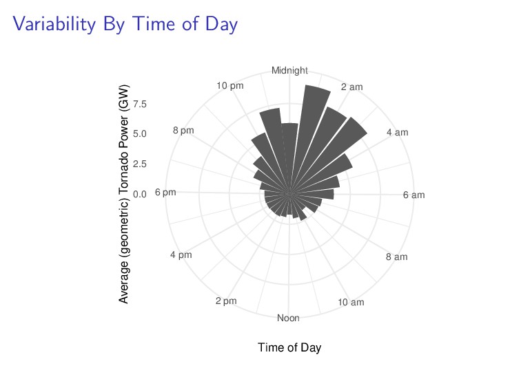
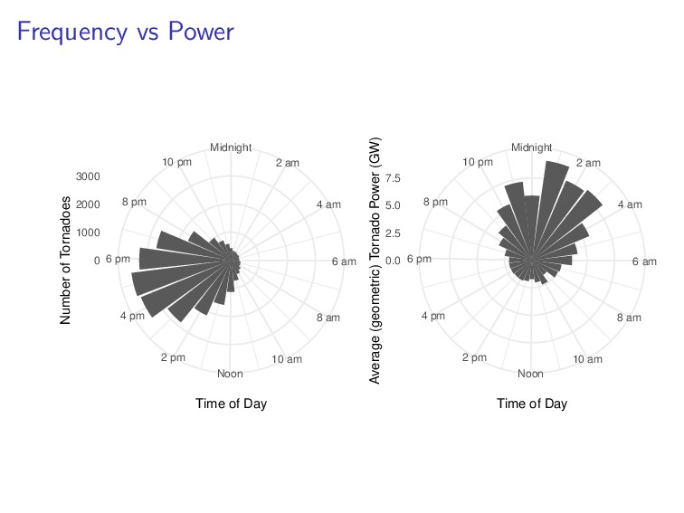
16. Frequency vs Power Midnight 2 am 4 am 6 am 8 am 10 am Noon 2 pm 4 pm 6 pm 8 pm 10 pm 0 1000 2000 3000 Number of Tornadoes Time of Day Midnight 2 am 4 am 6 am 8 am 10 am Noon 2 pm 4 pm 6 pm 8 pm 10 pm 0.0 2.5 5.0 7.5 Average (geometric) Tornado Power (GW) Time of Day
17. Variability By Month Jan Feb Mar Apr May Jun Jul Aug Sep Oct Nov Dec 0 2 4 6 Month Average (geometric) Tornado Power (GW)
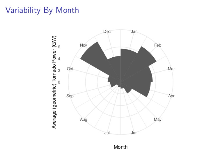
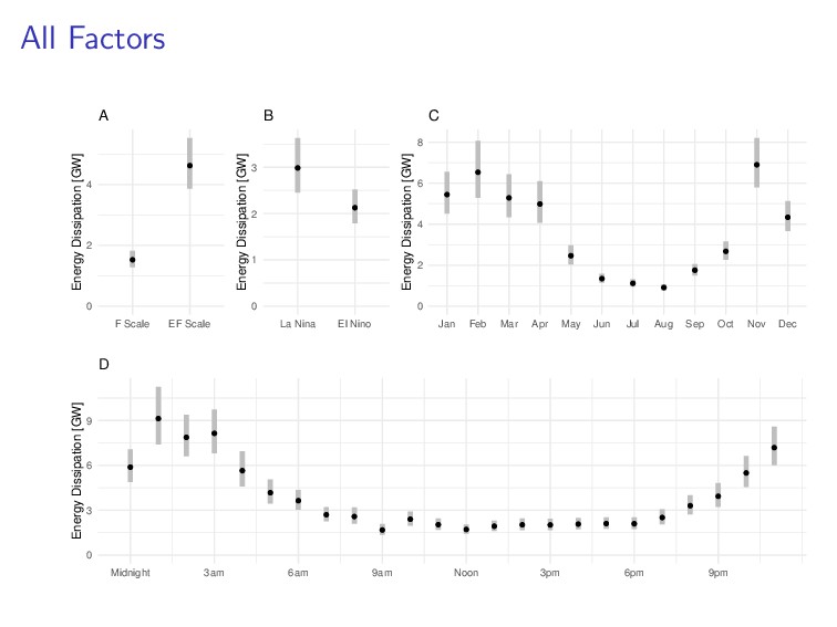
18. All Factors 0 1 2 3 0 2 4 6 8 Energy Dissipation [GW] Energy Dissipation [GW] 0 2 4 0 3 6 9 F Scale EF Scale La Nina El Nino Jan Feb Mar Apr May Jun Jul Aug Sep Oct Nov Dec Midnight 3am 6am 9am Noon 3pm 6pm 9pm Energy Dissipation [GW] Energy Dissipation [GW] A B C D
19. Statistical Model ln(P|P > 444000) = α + βYear Year+ βENSO ENSO+ βEF? EF?+ s(Month)+ s(Hour)
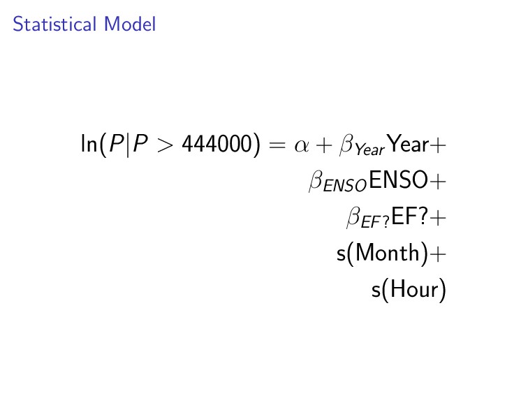
20. Fit the Model The model is fit using Bayesian simulations in the Stan computational framework (http://mc-stan.org/) accessed with brms package (B¨ urkner 2017) in R. To improve convergence and guard against over-fitting, we specify mildly informative conservative priors. Data & code: https://github.com/jelsner/tor-pwr-up
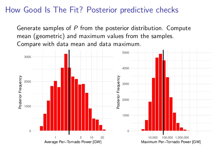
21. How Good Is The Fit? Posterior predictive checks Generate samples of P from the posterior distribution. Compute mean (geometric) and maximum values from the samples. Compare with data mean and data maximum. 0 1000 2000 3000 1 5 10 20 Average Per−Tornado Power [GW] Posterior Frequency 0 1000 2000 3000 4000 5000 10,000 100,000 1,000,000 Maximum Per−Tornado Power [GW] Posterior Frequency
22. Conditional Monthly Effect 0 50 100 150 Jan Feb Mar Apr May Jun Jul Aug Sep Oct Nov Dec Conditional Power [GW]
23. Fixed Effects Term Estimate Std. Error HDI1 βENSO −0.057 0.016 [−0.081 −0.031] βEF? 0.372 0.061 [0.282 0.476] βYear 0.051 0.004 [0.044 0.058] ENSO EF Rating Trend 0.75 1.00 1.25 1.50 1.75 Multiplicative Change 1Highest Density Interval (89%)
24. Conditional Trend Neutral ENSO conditions, after EF rating scaling change. 0.0 2.5 5.0 7.5 1995 2000 2005 2010 2015 Predicted Energy Dissipation [GW]
25. Modeled Trend by Month January February March April May June July August September October November December 1995 2005 2015 1995 2005 2015 1995 2005 2015 1995 2005 2015 1995 2005 2015 1995 2005 2015 1995 2005 2015 1995 2005 2015 1995 2005 2015 1995 2005 2015 1995 2005 2015 1995 2005 2015 0.1 1 10 100 1000 Energy Dissipation [GW]
26. Path Length & Width By Year 1995 2000 2005 2010 2015 1995 2000 2005 2010 2015 .1 1 10 100 1 10 100 Path Length (km) Path Width (m)
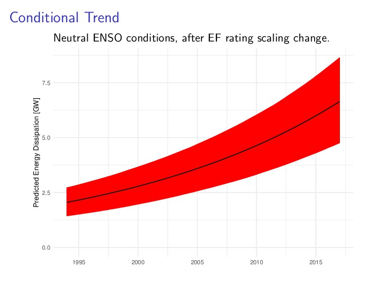
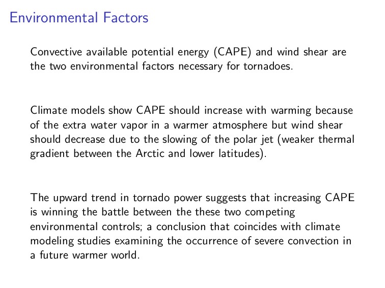
27. Environmental Factors Convective available potential energy (CAPE) and wind shear are the two environmental factors necessary for tornadoes. Climate models show CAPE should increase with warming because of the extra water vapor in a warmer atmosphere but wind shear should decrease due to the slowing of the polar jet (weaker thermal gradient between the Arctic and lower latitudes). The upward trend in tornado power suggests that increasing CAPE is winning the battle between the these two competing environmental controls; a conclusion that coincides with climate modeling studies examining the occurrence of severe convection in a future warmer world.
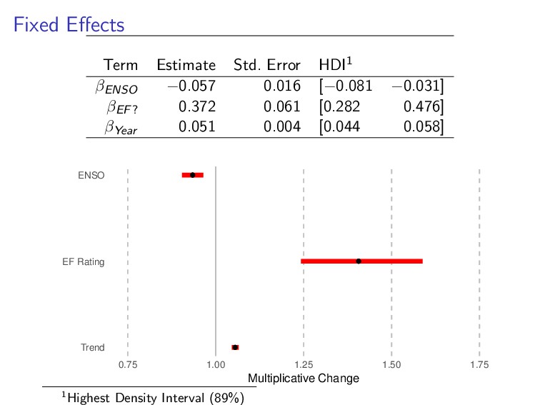
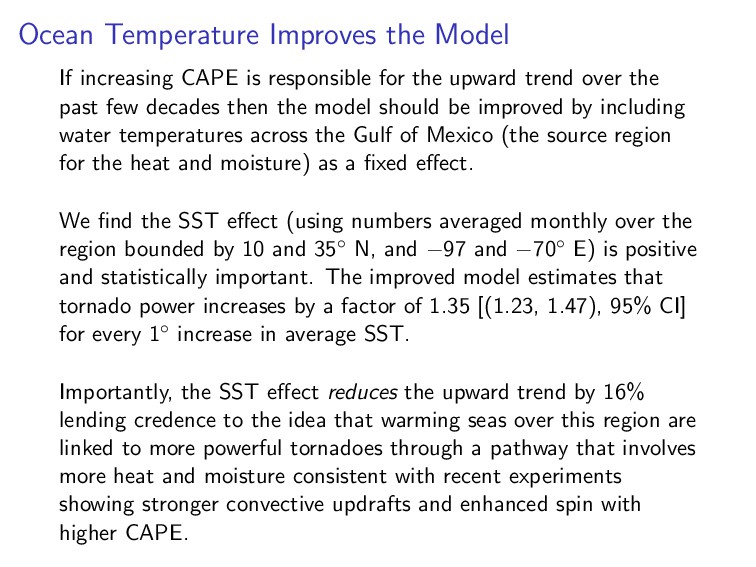
28. Ocean Temperature Improves the Model If increasing CAPE is responsible for the upward trend over the past few decades then the model should be improved by including water temperatures across the Gulf of Mexico (the source region for the heat and moisture) as a fixed effect. We find the SST effect (using numbers averaged monthly over the region bounded by 10 and 35◦ N, and −97 and −70◦ E) is positive and statistically important. The improved model estimates that tornado power increases by a factor of 1.35 [(1.23, 1.47), 95% CI] for every 1◦ increase in average SST. Importantly, the SST effect reduces the upward trend by 16% lending credence to the idea that warming seas over this region are linked to more powerful tornadoes through a pathway that involves more heat and moisture consistent with recent experiments showing stronger convective updrafts and enhanced spin with higher CAPE.
29. Why This Is Important: Casualty-Producing Tornadoes
30. Population Population (2012) 64 512 4096 32768 262144 2097152 16777216
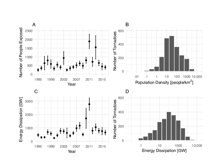
31. 0 500 1000 1500 2000 2500 1995 1999 2003 2007 2011 2015 Year Number of People Exposed A 0 200 400 600 .01 .1 1 10 100 1000 10,000 Population Density [people/km2] Number of Tornadoes B 0 1000 2000 3000 1995 1999 2003 2007 2011 2015 Year Energy Dissipation [GW] C 0 200 400 600 .1 10 1000 10,000 Energy Dissipation [GW] Number of Tornadoes D
32. May 22, 2011 Casualty-Producing Tornadoes Joplin, MO B B B B B B A A A A A A 10 100 1000 10 100 1000 Population Density [people/km2] Energy Dissipation [GW] 1 10 100 1000 Tornado Casualties
33. 2011 Casualty-Producing Tornadoes Joplin, MO .1 1 10 100 1000 10,000 100,000 1 10 100 1000 Population Density [people/km2] Energy Dissipation [GW] 1 10 100 1000 Tornado Casualties
34. All Casualty-Producing Tornadoes Joplin, MO .01 .1 1 10 100 1000 10,000 100,000 .01 .1 1 10 100 1000 10,000 Population Density [people/km2] Energy Dissipation [GW] 1 10 100 1000 Tornado Casualties
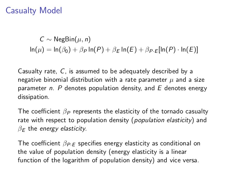
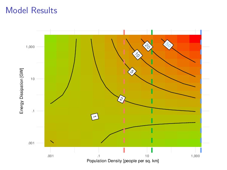
35. Casualty Model C ∼ NegBin(µ, n) ln(µ) = ln(β0) + βP ln(P) + βE ln(E) + βP·E [ln(P) · ln(E)] Casualty rate, C, is assumed to be adequately described by a negative binomial distribution with a rate parameter µ and a size parameter n. P denotes population density, and E denotes energy dissipation. The coefficient βP represents the elasticity of the tornado casualty rate with respect to population density (population elasticity) and βE the energy elasticity. The coefficient βP·E specifies energy elasticity as conditional on the value of population density (energy elasticity is a linear function of the logarithm of population density) and vice versa.
36. Model Results 1 2 5 10 20 50 .001 .1 10 1,000 .001 .1 10 1,000 Population Density [people per sq. km] Energy Dissipation [GW]
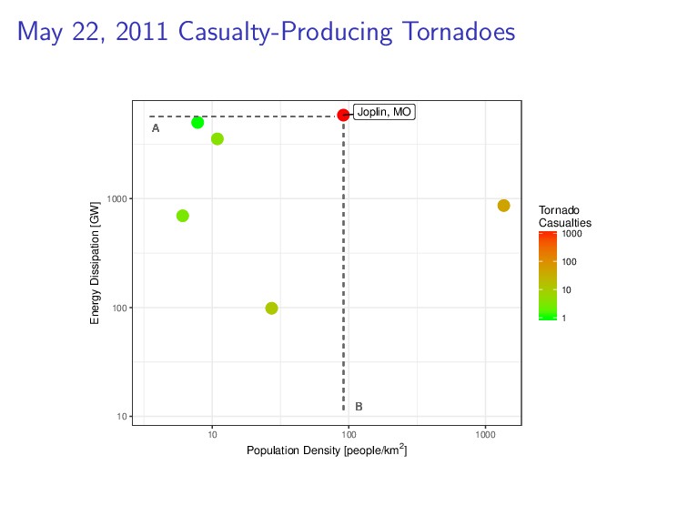
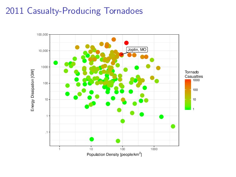
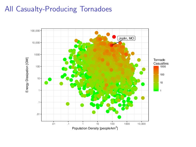
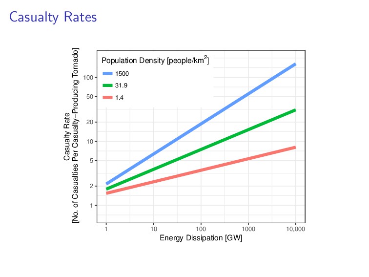
37. Casualty Rates 1 2 5 10 20 50 100 1 10 100 1000 10,000 Energy Dissipation [GW] Casualty Rate [No. of Casualties Per Casualty−Producing Tornado] Population Density [people/km2] 1500 31.9 1.4
38. Summary Tornado power has increased over the past few decades likely due to greater convective energy from hotter oceans. This means an increased potential for more casualties especially as more people are placed in harm’s way. Thank you for your attention. What questions do you have?