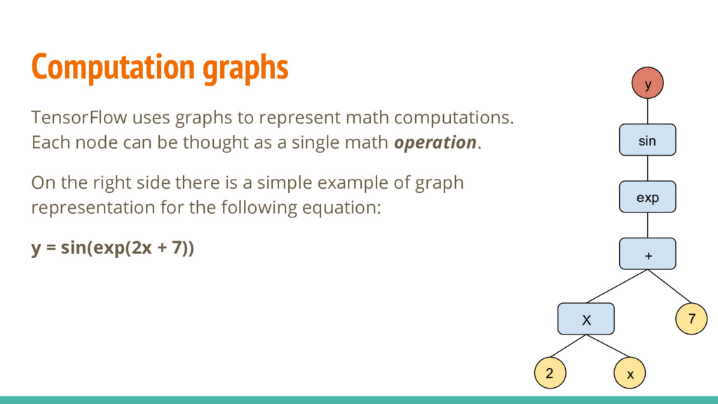
node can be thought as a single math operation. On the right side there is a simple example of graph representation for the following equation: y = sin(exp(2x + 7)) y sin exp + X 2 x 7
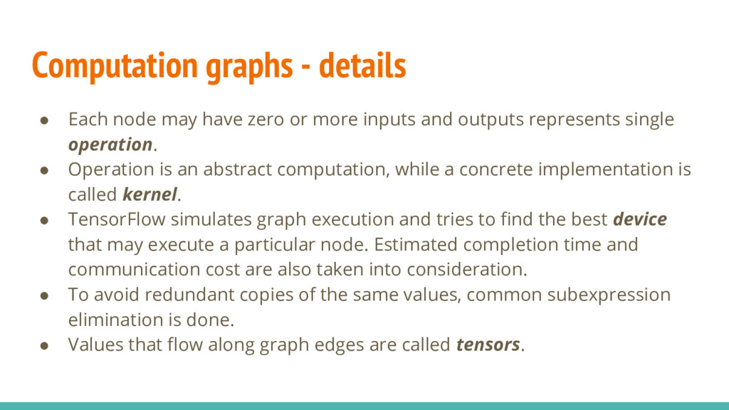
or more inputs and outputs represents single operation. • Operation is an abstract computation, while a concrete implementation is called kernel. • TensorFlow simulates graph execution and tries to find the best device that may execute a particular node. Estimated completion time and communication cost are also taken into consideration. • To avoid redundant copies of the same values, common subexpression elimination is done. • Values that flow along graph edges are called tensors.
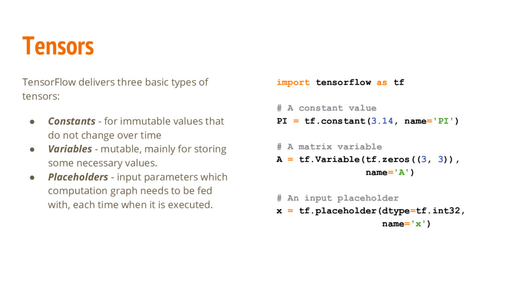
- for immutable values that do not change over time • Variables - mutable, mainly for storing some necessary values. • Placeholders - input parameters which computation graph needs to be fed with, each time when it is executed. import tensorflow as tf # A constant value PI = tf.constant(3.14, name='PI') # A matrix variable A = tf.Variable(tf.zeros((3, 3)), name='A') # An input placeholder x = tf.placeholder(dtype=tf.int32, name='x')
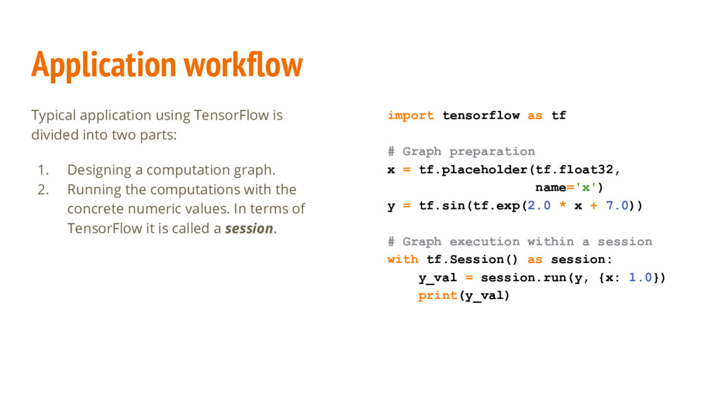
parts: 1. Designing a computation graph. 2. Running the computations with the concrete numeric values. In terms of TensorFlow it is called a session. import tensorflow as tf # Graph preparation x = tf.placeholder(tf.float32, name='x') y = tf.sin(tf.exp(2.0 * x + 7.0)) # Graph execution within a session with tf.Session() as session: y_val = session.run(y, {x: 1.0}) print(y_val)
monitor the execution of a computation graph, observe the changes of variable values over time. In order to use TensorBoard, an application has to be adapted to write logs into given directory. These logs can be visualized via browser application then.
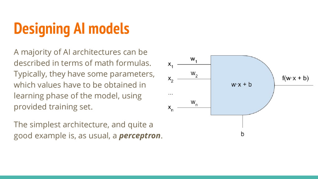
described in terms of math formulas. Typically, they have some parameters, which values have to be obtained in learning phase of the model, using provided training set. The simplest architecture, and quite a good example is, as usual, a perceptron.
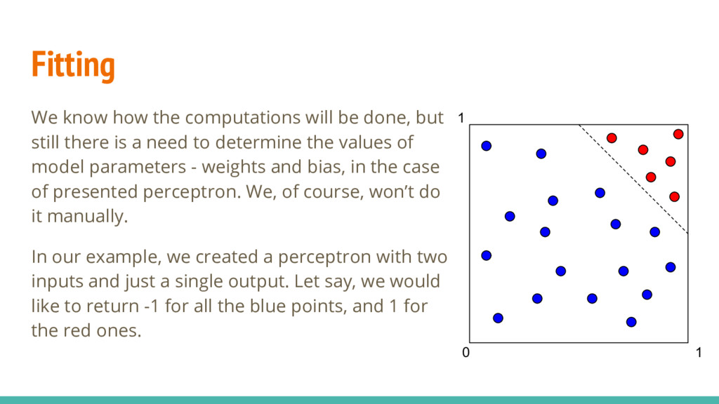
still there is a need to determine the values of model parameters - weights and bias, in the case of presented perceptron. We, of course, won’t do it manually. In our example, we created a perceptron with two inputs and just a single output. Let say, we would like to return -1 for all the blue points, and 1 for the red ones. 0 1 1
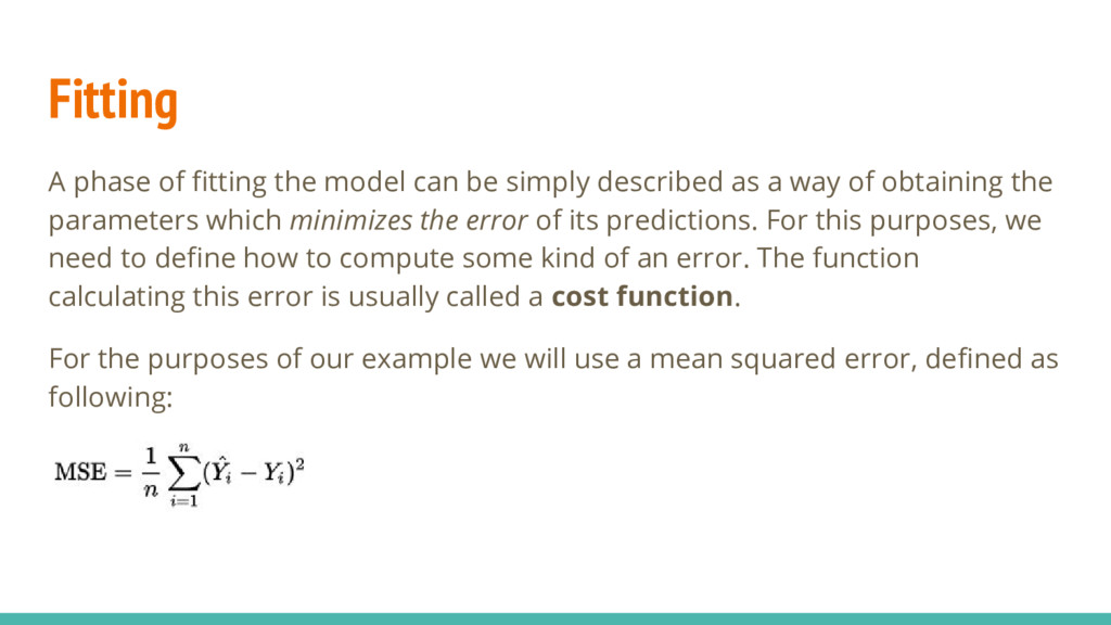
described as a way of obtaining the parameters which minimizes the error of its predictions. For this purposes, we need to define how to compute some kind of an error. The function calculating this error is usually called a cost function. For the purposes of our example we will use a mean squared error, defined as following:
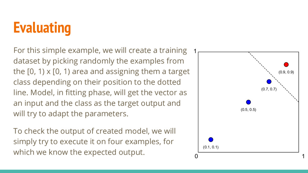
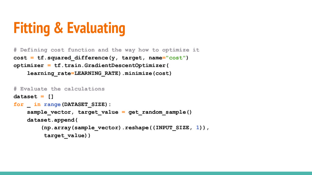
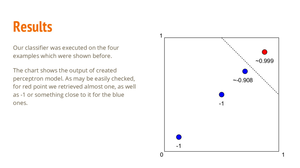
dataset by picking randomly the examples from the [0, 1) x [0, 1) area and assigning them a target class depending on their position to the dotted line. Model, in fitting phase, will get the vector as an input and the class as the target output and will try to adapt the parameters. To check the output of created model, we will simply try to execute it on four examples, for which we know the expected output. 0 1 1 (0.1, 0.1) (0.5, 0.5) (0.7, 0.7) (0.9, 0.9)
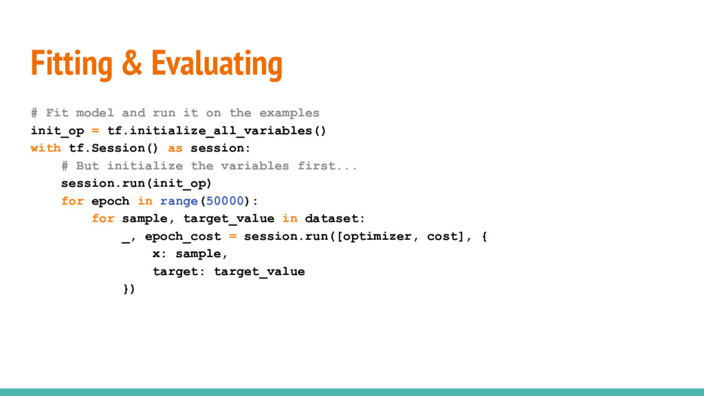
the examples init_op = tf.initialize_all_variables() with tf.Session() as session: # But initialize the variables first... session.run(init_op) for epoch in range(50000): for sample, target_value in dataset: _, epoch_cost = session.run([optimizer, cost], { x: sample, target: target_value })
was executed on the four examples which were shown before. The chart shows the output of created perceptron model. As may be easily checked, for red point we retrieved almost one, as well as -1 or something close to it for the blue ones.
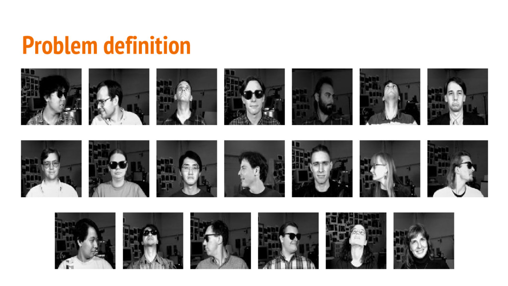
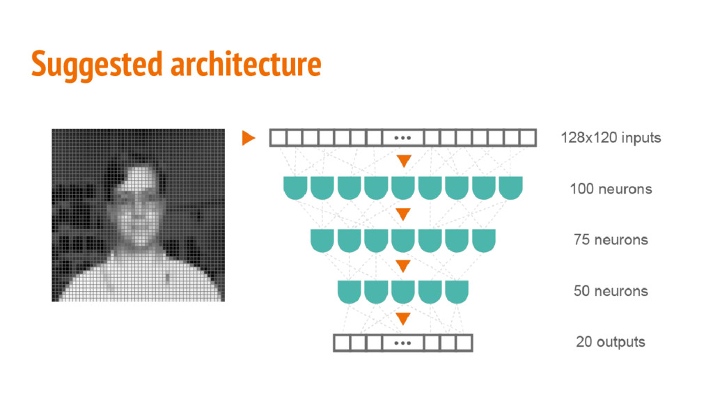
photos of 20 people. For each person there are up to 32 images taken with different pose, emotion and with or without sunglasses. Our goal will be to recognize a person from the photo using AI architecture. For the sake of laziness, we won’t even try to retrieve any features from the images, but will just try to prepare a solution working on the raw images.
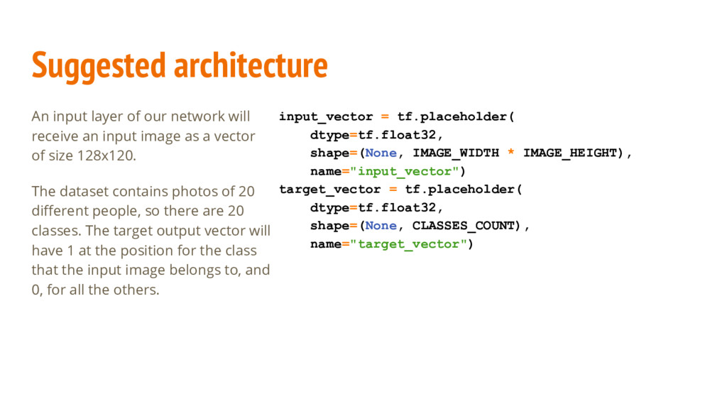
an input image as a vector of size 128x120. The dataset contains photos of 20 different people, so there are 20 classes. The target output vector will have 1 at the position for the class that the input image belongs to, and 0, for all the others. input_vector = tf.placeholder( dtype=tf.float32, shape=(None, IMAGE_WIDTH * IMAGE_HEIGHT), name="input_vector") target_vector = tf.placeholder( dtype=tf.float32, shape=(None, CLASSES_COUNT), name="target_vector")
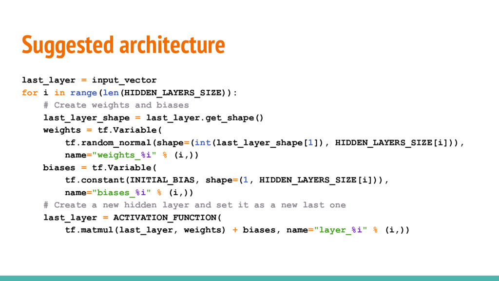
Create weights and biases last_layer_shape = last_layer.get_shape() weights = tf.Variable( tf.random_normal(shape=(int(last_layer_shape[1]), HIDDEN_LAYERS_SIZE[i])), name="weights_%i" % (i,)) biases = tf.Variable( tf.constant(INITIAL_BIAS, shape=(1, HIDDEN_LAYERS_SIZE[i])), name="biases_%i" % (i,)) # Create a new hidden layer and set it as a new last one last_layer = ACTIVATION_FUNCTION( tf.matmul(last_layer, weights) + biases, name="layer_%i" % (i,))
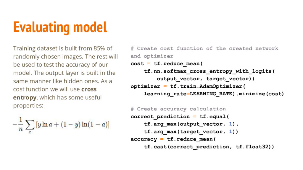
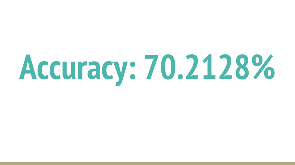
chosen images. The rest will be used to test the accuracy of our model. The output layer is built in the same manner like hidden ones. As a cost function we will use cross entropy, which has some useful properties: # Create cost function of the created network and optimizer cost = tf.reduce_mean( tf.nn.softmax_cross_entropy_with_logits( output_vector, target_vector)) optimizer = tf.train.AdamOptimizer( learning_rate=LEARNING_RATE).minimize(cost) # Create accuracy calculation correct_prediction = tf.equal( tf.arg_max(output_vector, 1), tf.arg_max(target_vector, 1)) accuracy = tf.reduce_mean( tf.cast(correct_prediction, tf.float32))