DAT630/2017 [DM] Frequent Itemsets and Association Rule Mining

University of Stavanger, DAT630, 2017 Autumn
lecture by Vinay Setty

Transcript

1. Frequent Itemsets and Association Rule Mining Vinay Setty vinay.j.setty@uis.no Slides credit: http://www.mmds.org/
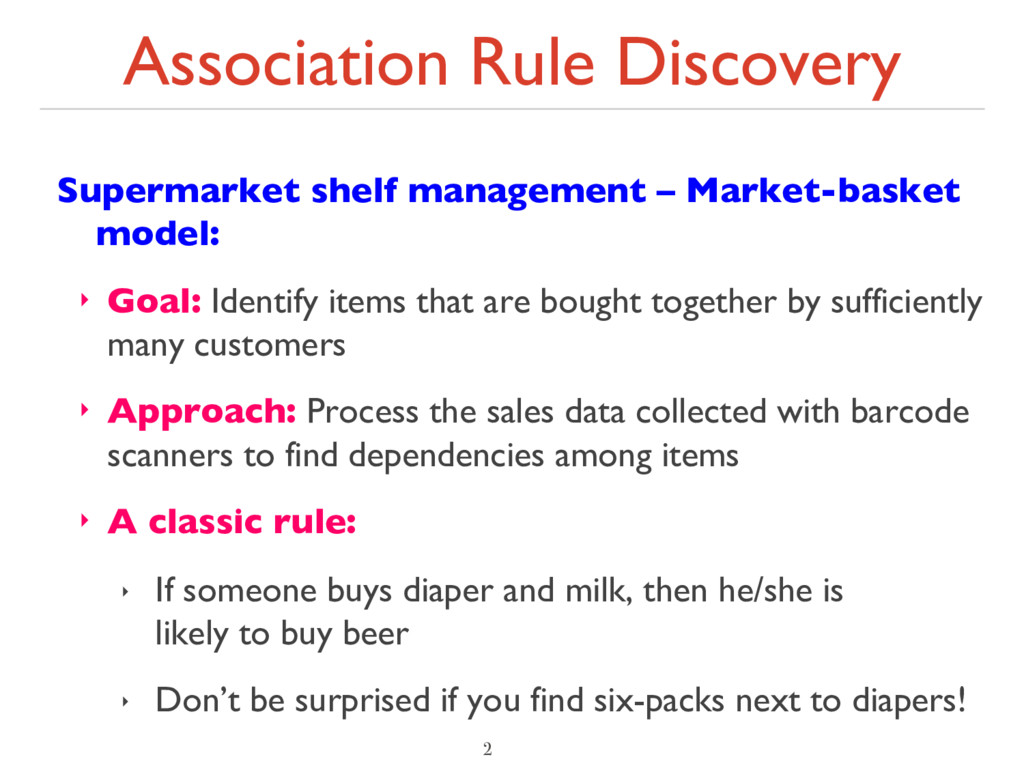
2. Association Rule Discovery Supermarket shelf management – Market-basket model: ‣ Goal: Identify items that are bought together by sufficiently many customers ‣ Approach: Process the sales data collected with barcode scanners to find dependencies among items ‣ A classic rule: ‣ If someone buys diaper and milk, then he/she is likely to buy beer ‣ Don’t be surprised if you find six-packs next to diapers! 2
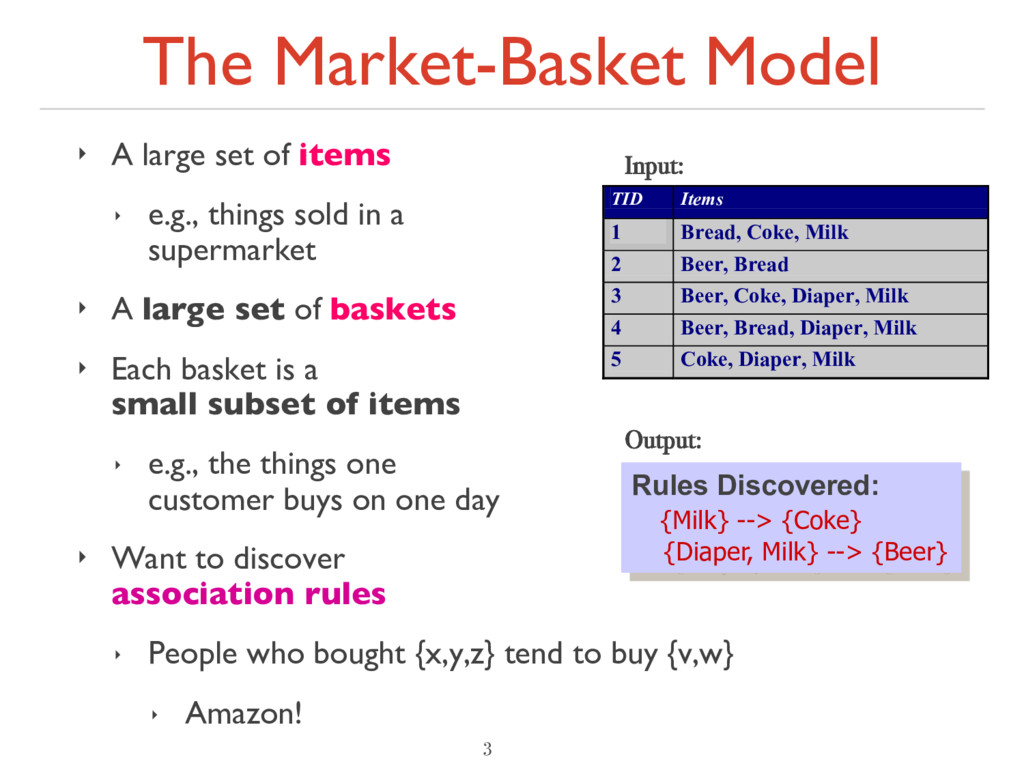
3. The Market-Basket Model ‣ A large set of items ‣ e.g., things sold in a supermarket ‣ A large set of baskets ‣ Each basket is a small subset of items ‣ e.g., the things one customer buys on one day ‣ Want to discover association rules ‣ People who bought {x,y,z} tend to buy {v,w} ‣ Amazon! 3 Rules Discovered: {Milk} --> {Coke} {Diaper, Milk} --> {Beer} TID Items 1 Bread, Coke, Milk 2 Beer, Bread 3 Beer, Coke, Diaper, Milk 4 Beer, Bread, Diaper, Milk 5 Coke, Diaper, Milk Input: Output:
4. Applications – (1) ‣ Items = products; Baskets = sets of products someone bought in one trip to the store ‣ Real market baskets: Chain stores keep TBs of data about what customers buy together ‣ Tells how typical customers navigate stores, lets them position tempting items ‣ Suggests tie-in “tricks”, e.g., run sale on diapers and raise the price of beer ‣ Need the rule to occur frequently, or no $$’s ‣ Amazon’s people who bought X also bought Y 4
5. Applications – (2) ‣ Baskets = sentences; Items = documents containing those sentences ‣ Items that appear together too often could represent plagiarism ‣ Notice items do not have to be “in” baskets ‣ Baskets = patients; Items = drugs & side-effects ‣ Has been used to detect combinations of drugs that result in particular side-effects ‣ But requires extension: Absence of an item needs to be observed as well as presence 5
6. More generally ‣ A general many-to-many mapping (association) between two kinds of things ‣ But we ask about connections among “items”, not “baskets” ‣ For example: ‣ Finding communities in graphs (e.g., Twitter) 6
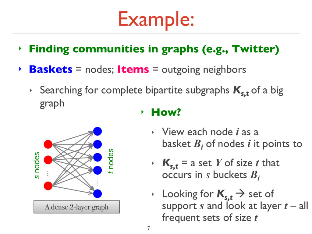
7. Example: ‣ Finding communities in graphs (e.g., Twitter) ‣ Baskets = nodes; Items = outgoing neighbors ‣ Searching for complete bipartite subgraphs Ks,t of a big graph 7 ‣ How? ‣ View each node i as a basket Bi of nodes i it points to ‣ Ks,t = a set Y of size t that occurs in s buckets Bi ‣ Looking for Ks,t à set of support s and look at layer t – all frequent sets of size t … … A dense 2-layer graph s nodes t nodes
8. First: Define Frequent itemsets Association rules: Confidence, Support, Interestingness Then: Algorithms for finding frequent itemsets Finding frequent pairs A-Priori algorithm 8
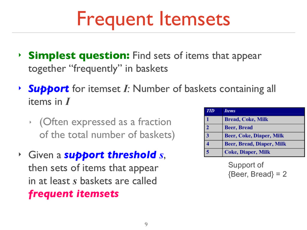
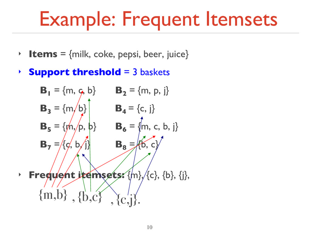
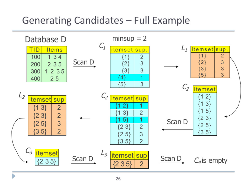
9. Frequent Itemsets ‣ Simplest question: Find sets of items that appear together “frequently” in baskets ‣ Support for itemset I: Number of baskets containing all items in I ‣ (Often expressed as a fraction of the total number of baskets) ‣ Given a support threshold s, then sets of items that appear in at least s baskets are called frequent itemsets 9 TID Items 1 Bread, Coke, Milk 2 Beer, Bread 3 Beer, Coke, Diaper, Milk 4 Beer, Bread, Diaper, Milk 5 Coke, Diaper, Milk Support of {Beer, Bread} = 2
10. Example: Frequent Itemsets ‣ Items = {milk, coke, pepsi, beer, juice} ‣ Support threshold = 3 baskets B1 = {m, c, b} B2 = {m, p, j} B3 = {m, b} B4 = {c, j} B5 = {m, p, b} B6 = {m, c, b, j} B7 = {c, b, j} B8 = {b, c} ‣ Frequent itemsets: {m}, {c}, {b}, {j}, 10 , {b,c} , {c,j}. {m,b}
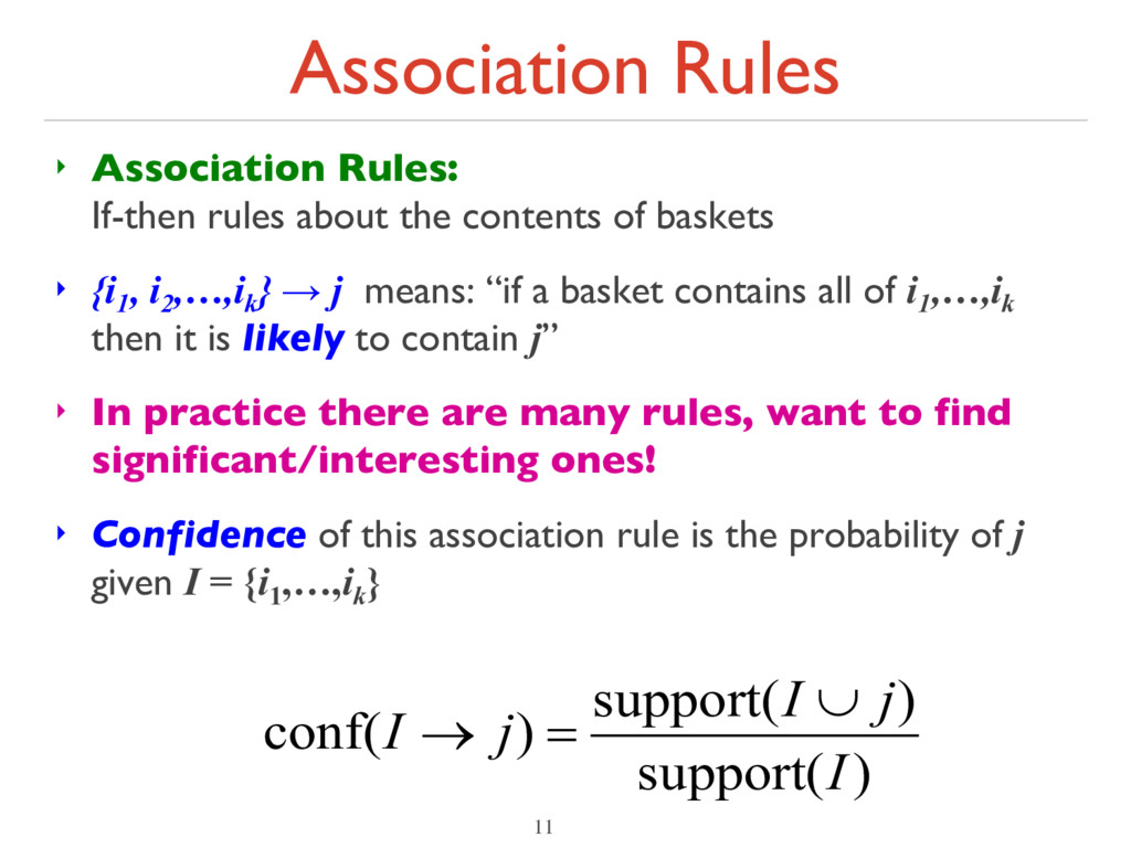
11. Association Rules ‣ Association Rules: If-then rules about the contents of baskets ‣ {i1 , i2 ,…,ik } → j means: “if a basket contains all of i1 ,…,ik then it is likely to contain j” ‣ In practice there are many rules, want to find significant/interesting ones! ‣ Confidence of this association rule is the probability of j given I = {i1 ,…,ik } 11 ) support( ) support( ) conf( I j I j I È = ®
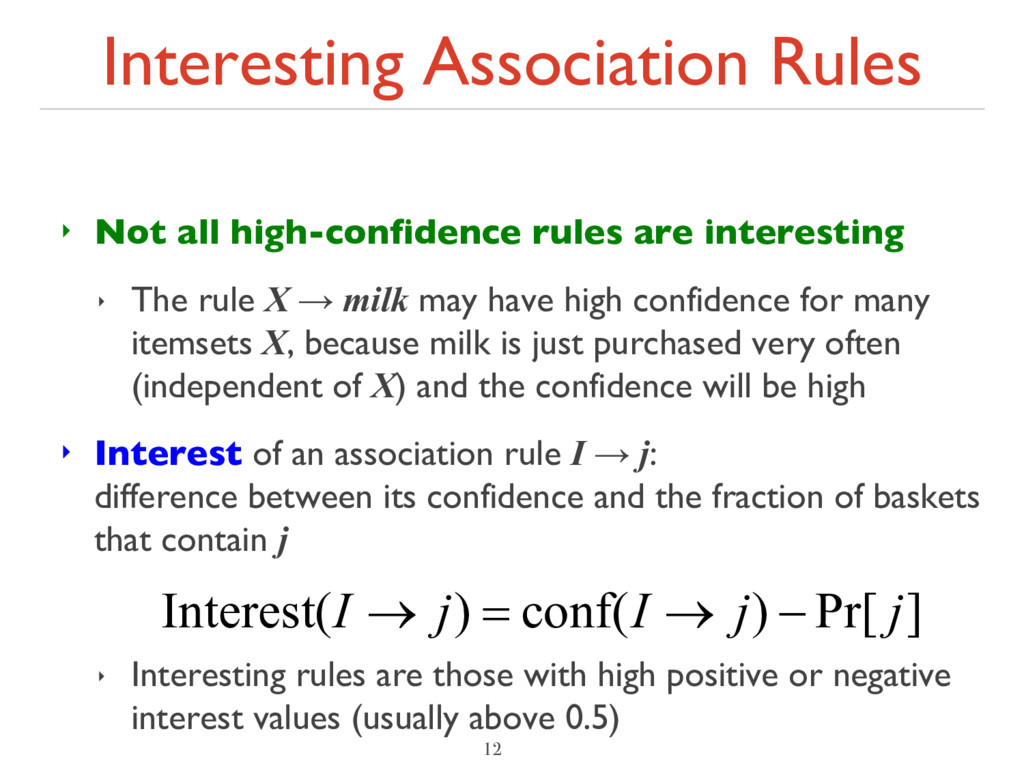
12. Interesting Association Rules ‣ Not all high-confidence rules are interesting ‣ The rule X → milk may have high confidence for many itemsets X, because milk is just purchased very often (independent of X) and the confidence will be high ‣ Interest of an association rule I → j: difference between its confidence and the fraction of baskets that contain j ‣ Interesting rules are those with high positive or negative interest values (usually above 0.5) 12 ] Pr[ ) conf( ) Interest( j j I j I - ® = ®
13. Example: Confidence and Interest B1 = {m, c, b} B2 = {m, p, j} B3 = {m, b} B4 = {c, j} B5 = {m, p, b} B6 = {m, c, b, j} B7 = {c, b, j} B8 = {b, c} ‣ Association rule: {m, b} →c ‣ Confidence = 2/4 = 0.5 ‣ Interest = |0.5 – 5/8| = 1/8 ‣ Item c appears in 5/8 of the baskets ‣ Rule is not very interesting! 13
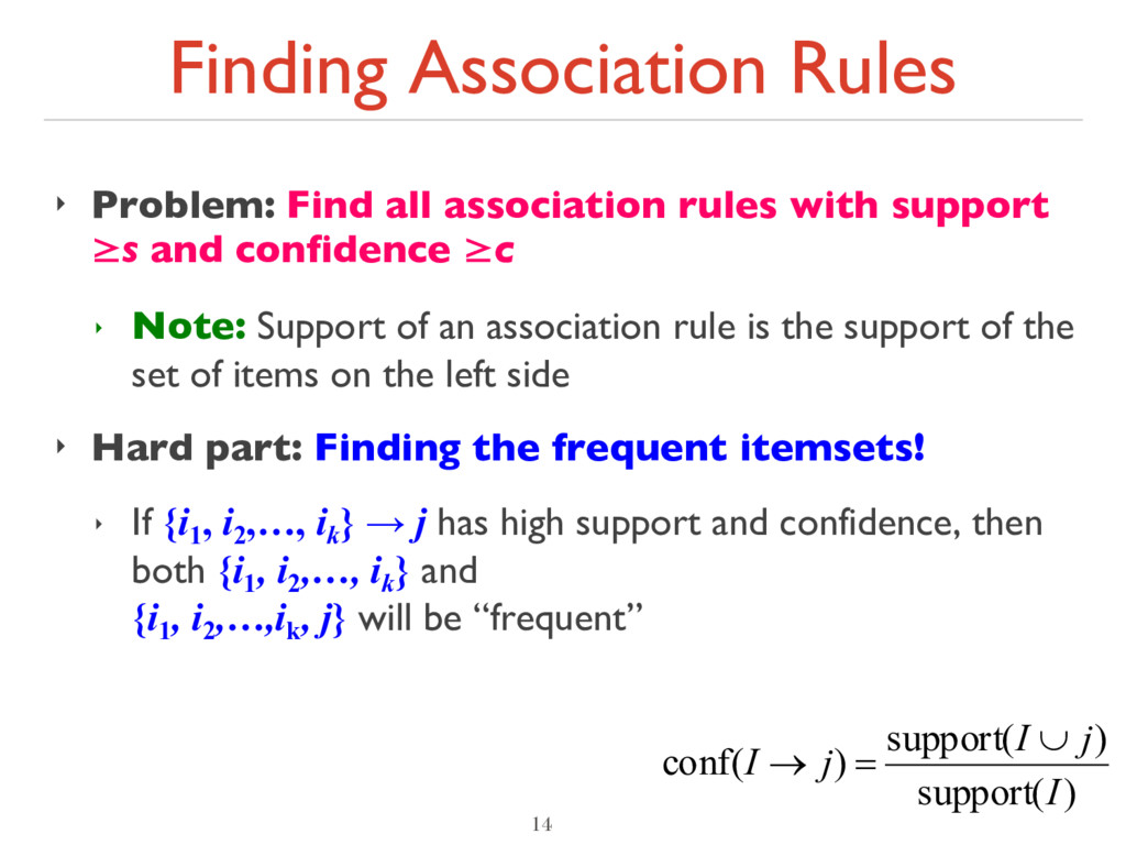
14. Finding Association Rules ‣ Problem: Find all association rules with support ≥s and confidence ≥c ‣ Note: Support of an association rule is the support of the set of items on the left side ‣ Hard part: Finding the frequent itemsets! ‣ If {i1 , i2 ,…, ik } → j has high support and confidence, then both {i1 , i2 ,…, ik } and {i1 , i2 ,…,ik , j} will be “frequent” 14 ) support( ) support( ) conf( I j I j I È = ®
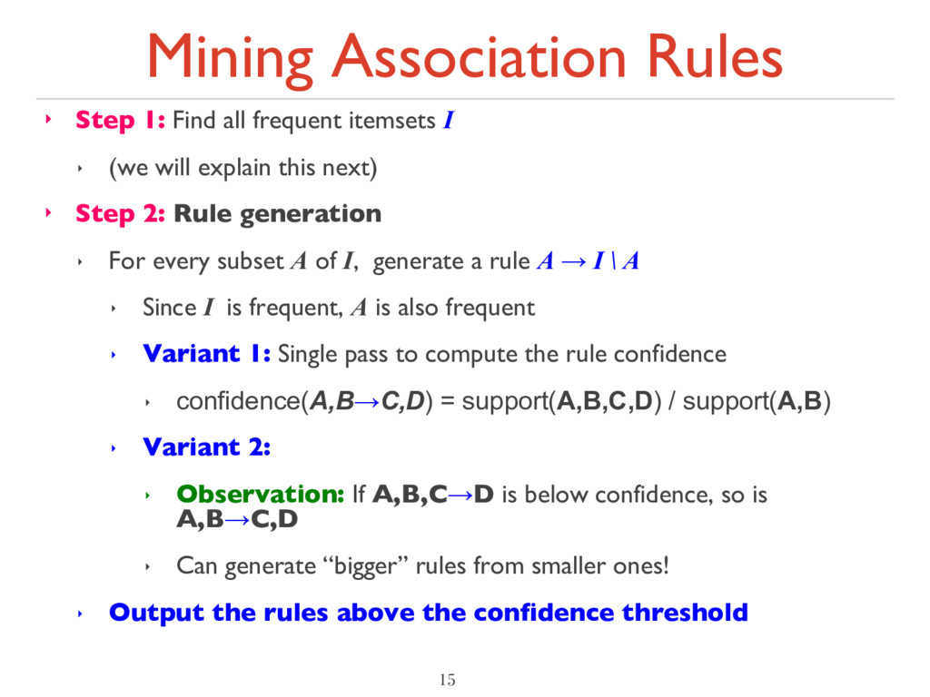
15. Mining Association Rules ‣ Step 1: Find all frequent itemsets I ‣ (we will explain this next) ‣ Step 2: Rule generation ‣ For every subset A of I, generate a rule A → I \ A ‣ Since I is frequent, A is also frequent ‣ Variant 1: Single pass to compute the rule confidence ‣ confidence(A,B→C,D) = support(A,B,C,D) / support(A,B) ‣ Variant 2: ‣ Observation: If A,B,C→D is below confidence, so is A,B→C,D ‣ Can generate “bigger” rules from smaller ones! ‣ Output the rules above the confidence threshold 15
16. Example B1 = {m, c, b} B2 = {m, p, j} B3 = {m, c, b, n} B4 = {c, j} B5 = {m, p, b} B6 = {m, c, b, j} B7 = {c, b, j} B8 = {b, c} ‣ Support threshold s = 3, confidence c = 0.75 ‣ 1) Frequent itemsets: ‣ {b,m} {b,c} {c,m} {c,j} {m,c,b} ‣ 2) Generate rules: ‣ b→m: c=4/6 b→c: c=5/6 b,c→m: c=3/5 ‣ m→b: c=4/5 … b,m→c: c=3/4 ‣ b→c,m: c=3/6 16
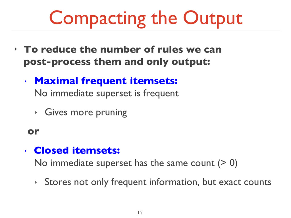
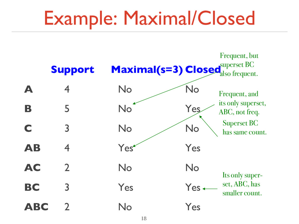
17. Compacting the Output ‣ To reduce the number of rules we can post-process them and only output: ‣ Maximal frequent itemsets: No immediate superset is frequent ‣ Gives more pruning or ‣ Closed itemsets: No immediate superset has the same count (> 0) ‣ Stores not only frequent information, but exact counts 17
18. Example: Maximal/Closed Support Maximal(s=3) Closed A 4 No No B 5 No Yes C 3 No No AB 4 Yes Yes AC 2 No No BC 3 Yes Yes ABC 2 No Yes 18 Frequent, but superset BC also frequent. Frequent, and its only superset, ABC, not freq. Superset BC has same count. Its only super- set, ABC, has smaller count.
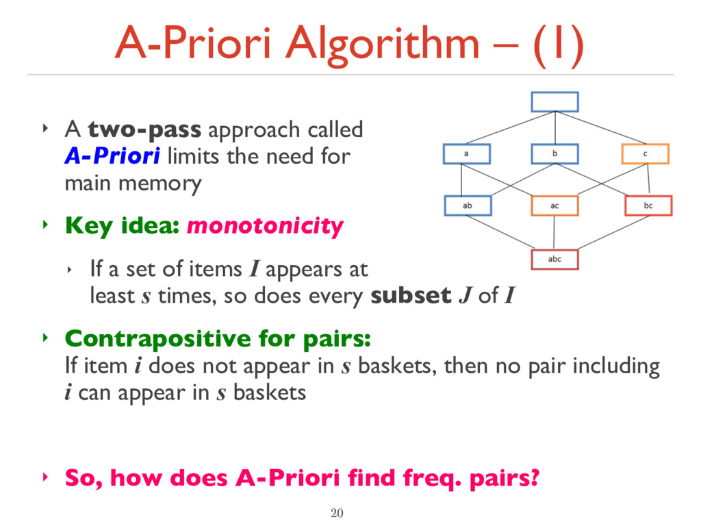
20. A-Priori Algorithm – (1) ‣ A two-pass approach called A-Priori limits the need for main memory ‣ Key idea: monotonicity ‣ If a set of items I appears at least s times, so does every subset J of I ‣ Contrapositive for pairs: If item i does not appear in s baskets, then no pair including i can appear in s baskets ‣ So, how does A-Priori find freq. pairs? 20
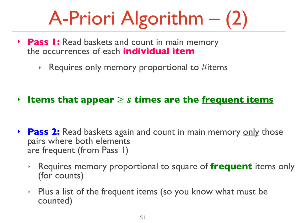
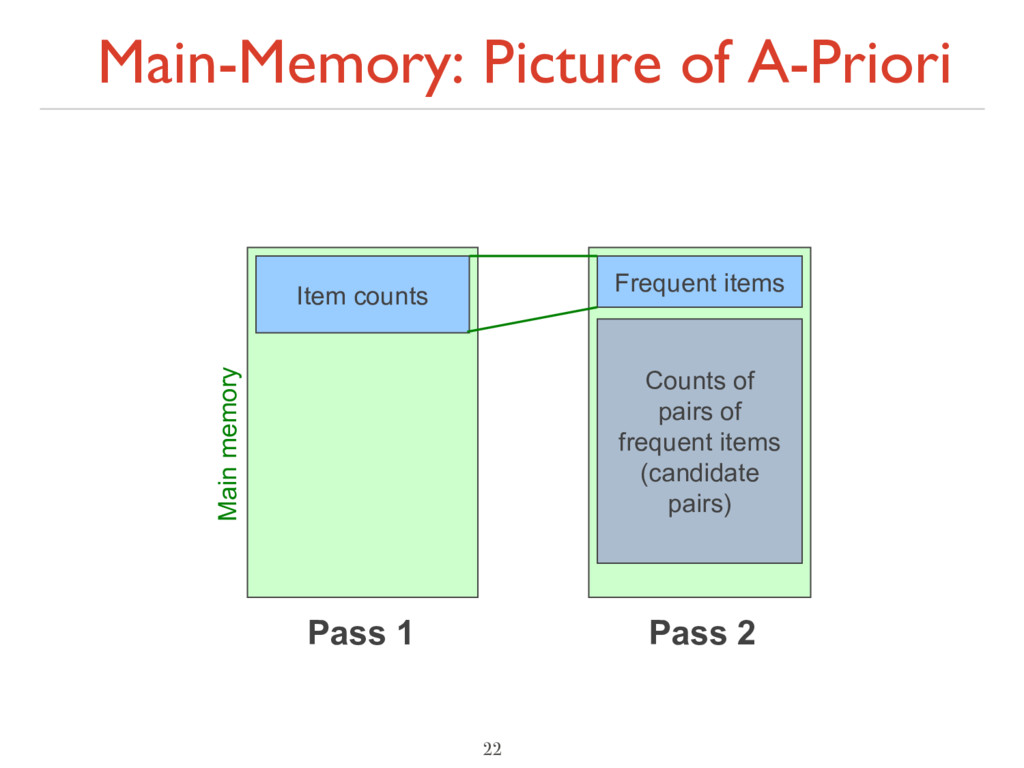
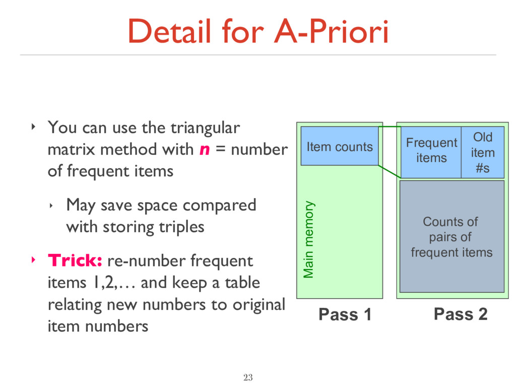
21. A-Priori Algorithm – (2) ‣ Pass 1: Read baskets and count in main memory the occurrences of each individual item ‣ Requires only memory proportional to #items ‣ Items that appear ≥ times are the frequent items ‣ Pass 2: Read baskets again and count in main memory only those pairs where both elements are frequent (from Pass 1) ‣ Requires memory proportional to square of frequent items only (for counts) ‣ Plus a list of the frequent items (so you know what must be counted) 21
22. Main-Memory: Picture of A-Priori 22 Item counts Pass 1 Pass 2 Frequent items Main memory Counts of pairs of frequent items (candidate pairs)
23. Detail for A-Priori ‣ You can use the triangular matrix method with n = number of frequent items ‣ May save space compared with storing triples ‣ Trick: re-number frequent items 1,2,… and keep a table relating new numbers to original item numbers 23 Item counts Pass 1 Pass 2 Counts of pairs of frequent items Frequent items Old item #s Main memory Counts of pairs of frequent items
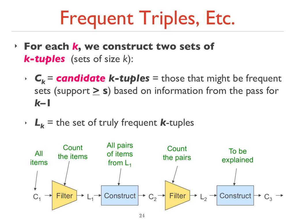
24. Frequent Triples, Etc. ‣ For each k, we construct two sets of k-tuples (sets of size k): ‣ Ck = candidate k-tuples = those that might be frequent sets (support > s) based on information from the pass for k–1 ‣ Lk = the set of truly frequent k-tuples 24 C1 L1 C2 L2 C3 Filter Filter Construct Construct All items All pairs of items from L1 Count the pairs To be explained Count the items
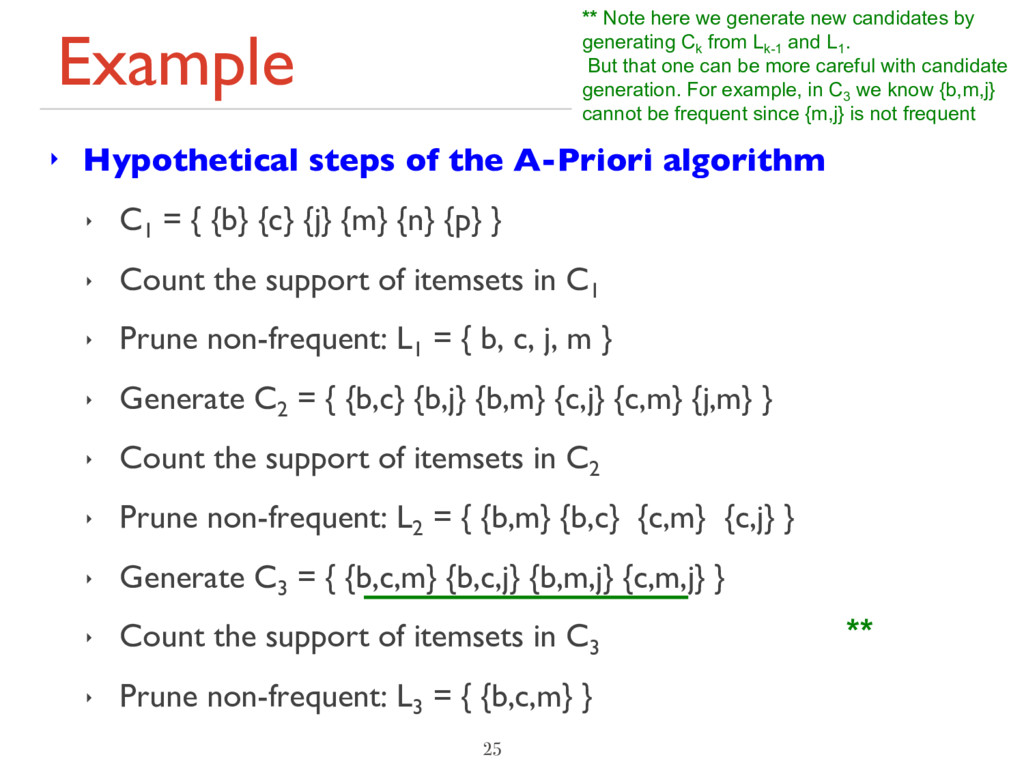
25. Example ‣ Hypothetical steps of the A-Priori algorithm ‣ C1 = { {b} {c} {j} {m} {n} {p} } ‣ Count the support of itemsets in C1 ‣ Prune non-frequent: L1 = { b, c, j, m } ‣ Generate C2 = { {b,c} {b,j} {b,m} {c,j} {c,m} {j,m} } ‣ Count the support of itemsets in C2 ‣ Prune non-frequent: L2 = { {b,m} {b,c} {c,m} {c,j} } ‣ Generate C3 = { {b,c,m} {b,c,j} {b,m,j} {c,m,j} } ‣ Count the support of itemsets in C3 ‣ Prune non-frequent: L3 = { {b,c,m} } 25 ** Note here we generate new candidates by generating Ck from Lk-1 and L1 . But that one can be more careful with candidate generation. For example, in C3 we know {b,m,j} cannot be frequent since {m,j} is not frequent **
26. Generating Candidates – Full Example Scan D itemset sup. {1} {2} {3} 2 3 3 {4} 1 {5} 3 C1 itemset sup {1 2} 1 {1 3} 2 {1 5} 1 {2 3} {2 5} {3 5} 2 3 2 C2 Scan D Scan D L3 itemset sup {2 3 5} 2 i t e m s e t s u p . {1} 2 {2} 3 {3} 3 {5} 3 L1 itemset sup {1 3} 2 {2 3} 2 {2 5} 3 {3 5} 2 L2 itemset {1 2} {1 3} {1 5} {2 3} {2 5} {3 5} C2 C3 itemset {2 3 5} TID Items 100 1 3 4 200 2 3 5 300 1 2 3 5 400 2 5 minsup = 2 Database D Scan D 26 C4 is empty
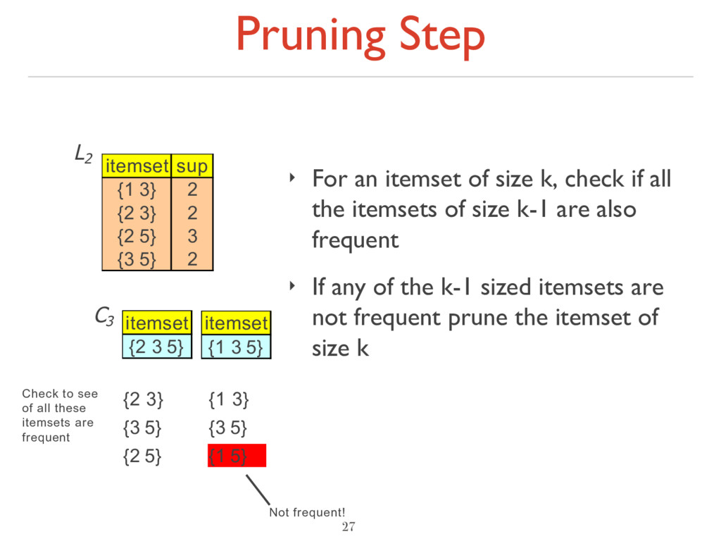
27. Pruning Step ‣ For an itemset of size k, check if all the itemsets of size k-1 are also frequent ‣ If any of the k-1 sized itemsets are not frequent prune the itemset of size k 27 itemset sup {1 3} 2 {2 3} 2 {2 5} 3 {3 5} 2 L2 C3 itemset {2 3 5} {2 3} {3 5} {2 5} Check to see of all these itemsets are frequent itemset {1 3 5} {1 3} {3 5} {1 5} Not frequent!
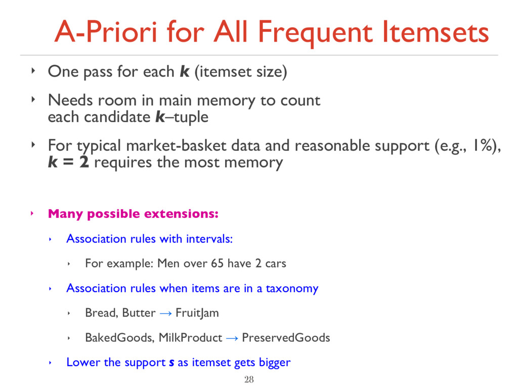
28. A-Priori for All Frequent Itemsets ‣ One pass for each k (itemset size) ‣ Needs room in main memory to count each candidate k–tuple ‣ For typical market-basket data and reasonable support (e.g., 1%), k = 2 requires the most memory ‣ Many possible extensions: ‣ Association rules with intervals: ‣ For example: Men over 65 have 2 cars ‣ Association rules when items are in a taxonomy ‣ Bread, Butter → FruitJam ‣ BakedGoods, MilkProduct → PreservedGoods ‣ Lower the support s as itemset gets bigger 28
30. Frequent Itemsets in < 2 Passes ‣ A-Priori takes k passes to find frequent itemsets of size k ‣ Can we use fewer passes? ‣ Use 2 or fewer passes for all sizes, but may miss some frequent itemsets ‣ Random sampling ‣ SON (Savasere, Omiecinski, and Navathe) ‣ Toivonen (see textbook) 30
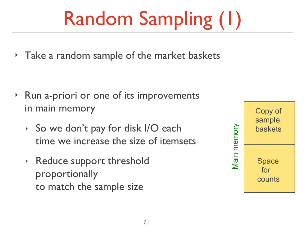
31. Random Sampling (1) ‣ Take a random sample of the market baskets ‣ Run a-priori or one of its improvements in main memory ‣ So we don’t pay for disk I/O each time we increase the size of itemsets ‣ Reduce support threshold proportionally to match the sample size 31 Copy of sample baskets Space for counts Main memory
32. Random Sampling (2) ‣ Optionally, verify that the candidate pairs are truly frequent in the entire data set by a second pass (avoid false positives) ‣ But you don’t catch sets frequent in the whole but not in the sample ‣ Smaller threshold, e.g., s/125, helps catch more truly frequent itemsets ‣ But requires more space 32
33. SON Algorithm – (1) ‣ Repeatedly read small subsets of the baskets into main memory and run an in-memory algorithm to find all frequent itemsets ‣ Note: we are not sampling, but processing the entire file in memory-sized chunks ‣ An itemset becomes a candidate if it is found to be frequent in any one or more subsets of the baskets. 33
34. SON Algorithm – (2) ‣ On a second pass, count all the candidate itemsets and determine which are frequent in the entire set ‣ Key “monotonicity” idea: an itemset cannot be frequent in the entire set of baskets unless it is frequent in at least one subset. 34
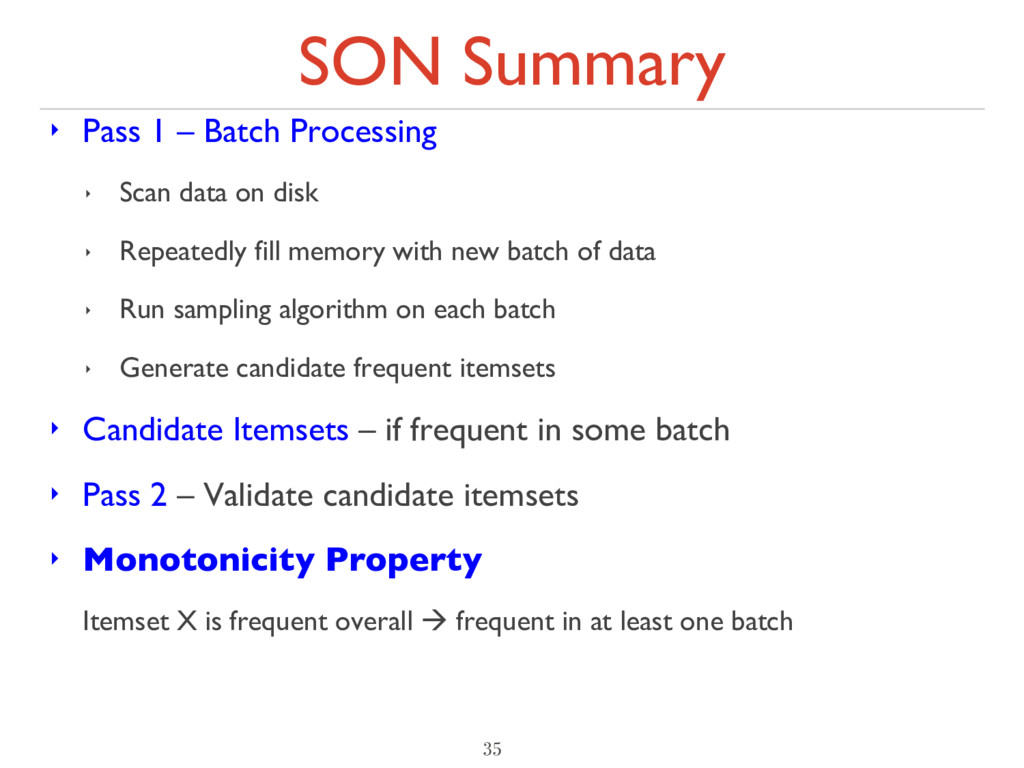
35. SON Summary 35 ‣ Pass 1 – Batch Processing ‣ Scan data on disk ‣ Repeatedly fill memory with new batch of data ‣ Run sampling algorithm on each batch ‣ Generate candidate frequent itemsets ‣ Candidate Itemsets – if frequent in some batch ‣ Pass 2 – Validate candidate itemsets ‣ Monotonicity Property Itemset X is frequent overall à frequent in at least one batch
36. SON – Distributed Version ‣ SON lends itself to distributed data mining ‣ Baskets distributed among many nodes ‣ Compute frequent itemsets at each node ‣ Distribute candidates to all nodes ‣ Accumulate the counts of all candidates 36
37. SON: Map/Reduce ‣ Phase 1: Find candidate itemsets ‣ Map? ‣ Reduce? ‣ Phase 2: Find true frequent itemsets ‣ Map? ‣ Reduce? 37
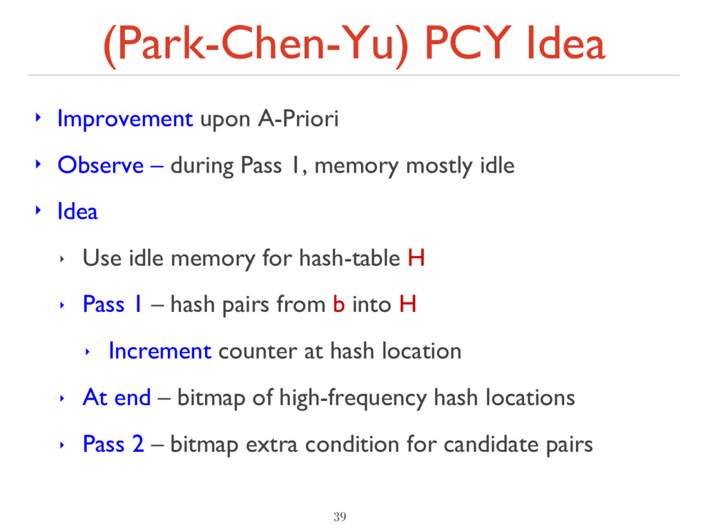
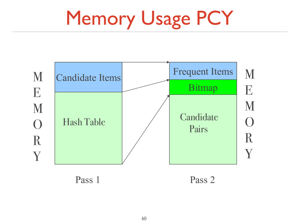
39. (Park-Chen-Yu) PCY Idea 39 ‣ Improvement upon A-Priori ‣ Observe – during Pass 1, memory mostly idle ‣ Idea ‣ Use idle memory for hash-table H ‣ Pass 1 – hash pairs from b into H ‣ Increment counter at hash location ‣ At end – bitmap of high-frequency hash locations ‣ Pass 2 – bitmap extra condition for candidate pairs
40. Memory Usage PCY 40 Candidate Items Pass 1 Pass 2 M E M O R Y M E M O R Y Hash Table Frequent Items Bitmap Candidate Pairs
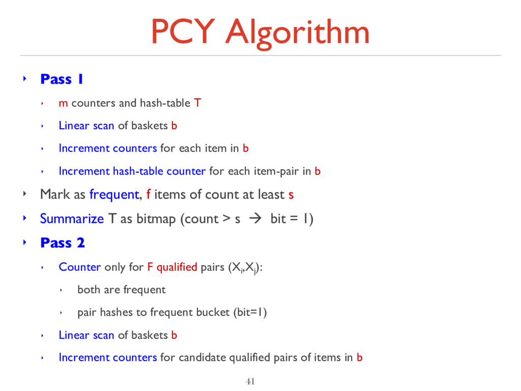
41. PCY Algorithm ‣ Pass 1 ‣ m counters and hash-table T ‣ Linear scan of baskets b ‣ Increment counters for each item in b ‣ Increment hash-table counter for each item-pair in b ‣ Mark as frequent, f items of count at least s ‣ Summarize T as bitmap (count > s à bit = 1) ‣ Pass 2 ‣ Counter only for F qualified pairs (Xi ,Xj ): ‣ both are frequent ‣ pair hashes to frequent bucket (bit=1) ‣ Linear scan of baskets b ‣ Increment counters for candidate qualified pairs of items in b 41
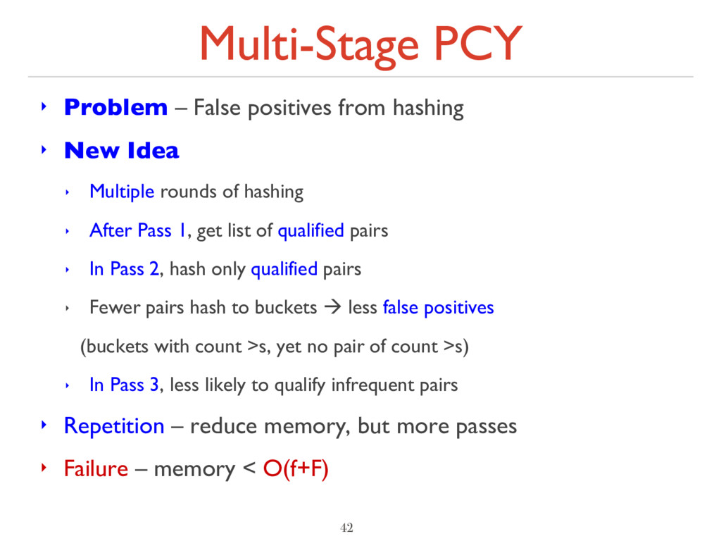
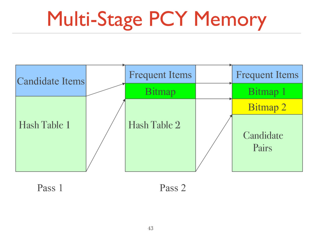
42. Multi-Stage PCY ‣ Problem – False positives from hashing ‣ New Idea ‣ Multiple rounds of hashing ‣ After Pass 1, get list of qualified pairs ‣ In Pass 2, hash only qualified pairs ‣ Fewer pairs hash to buckets à less false positives (buckets with count >s, yet no pair of count >s) ‣ In Pass 3, less likely to qualify infrequent pairs ‣ Repetition – reduce memory, but more passes ‣ Failure – memory < O(f+F) 42
43. Multi-Stage PCY Memory 43 Candidate Items Pass 1 Pass 2 Hash Table 1 Frequent Items Bitmap Frequent Items Bitmap 1 Bitmap 2 Candidate Pairs Hash Table 2
44. Literature ‣ Mining of Massive Datasets Jure Leskovec, Anand Rajaraman, Jeff Ullman, Chapter 6 ‣ http://mmds.org http://infolab.stanford.edu/~ullman/mmds/ch6.pdf 44