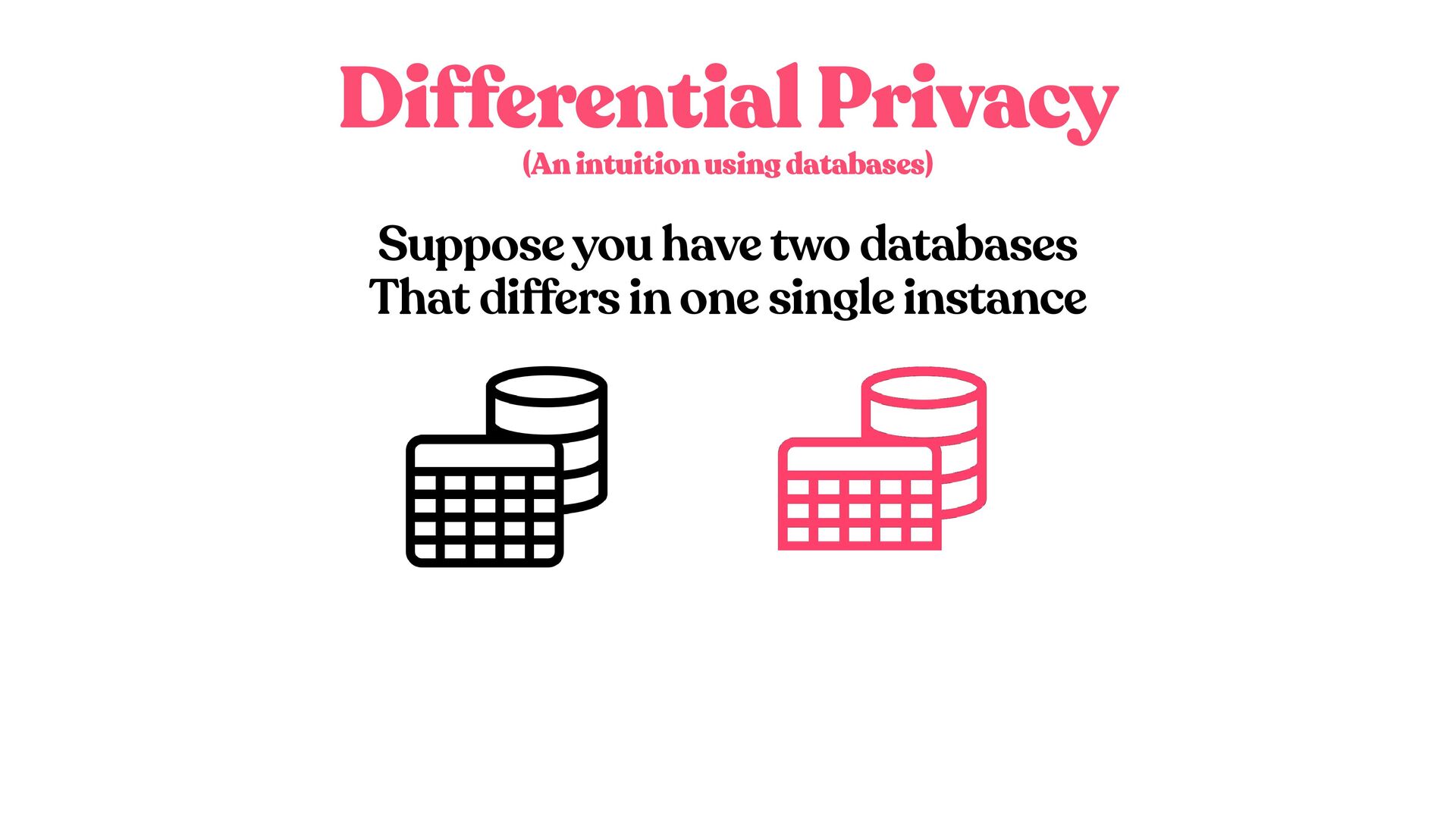
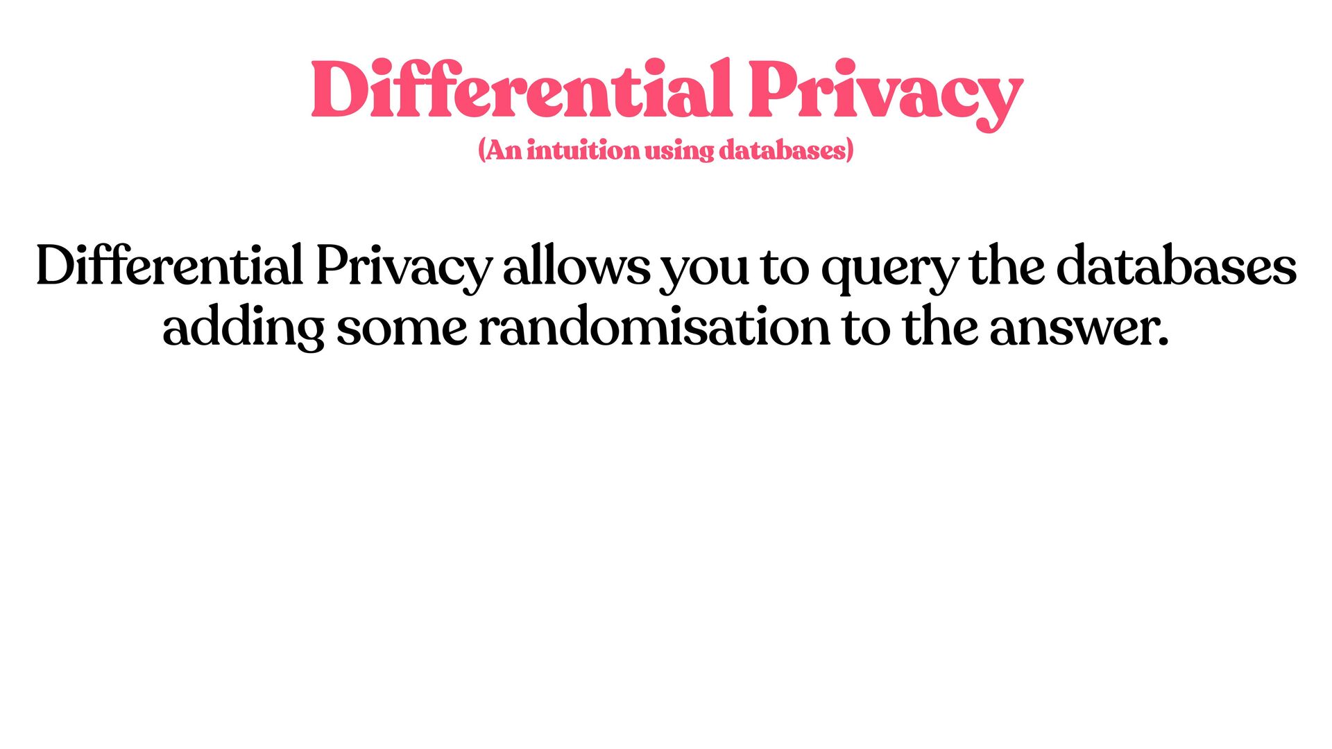
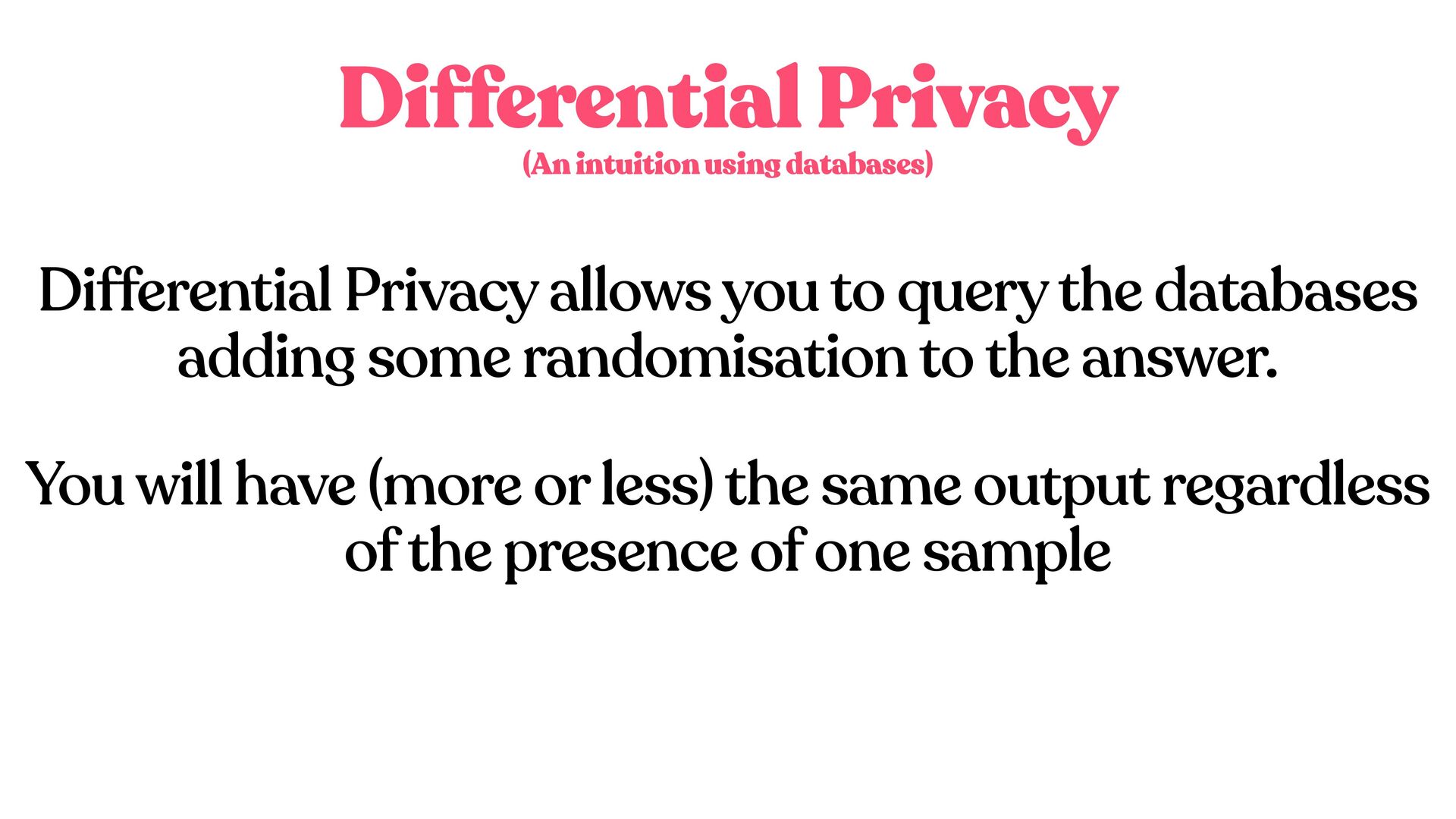
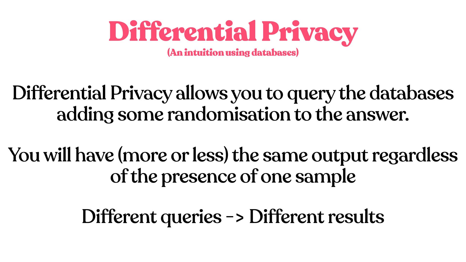
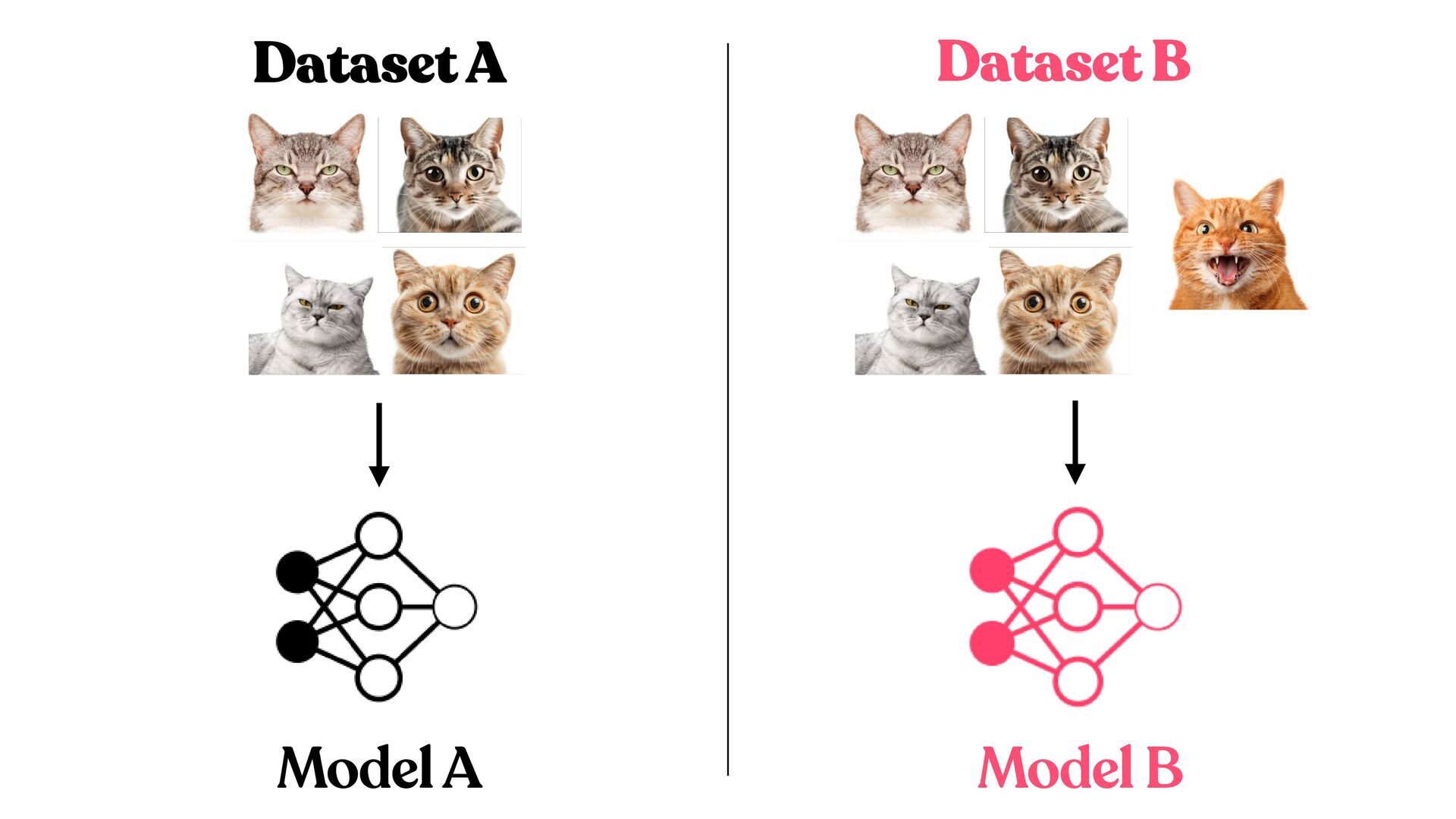
adding some randomisation to the answer. (An intuition using databases) You will have (more or less) the same output regardless of the presence of one sample
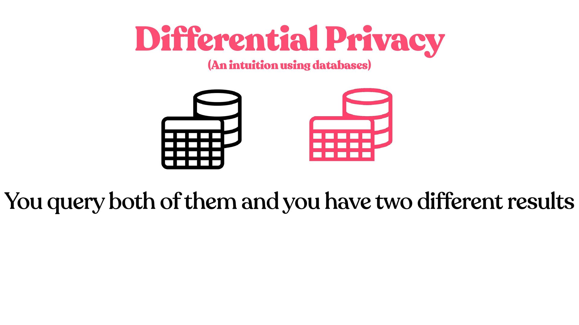
adding some randomisation to the answer. (An intuition using databases) You will have (more or less) the same output regardless of the presence of one sample Different queries -> Different results
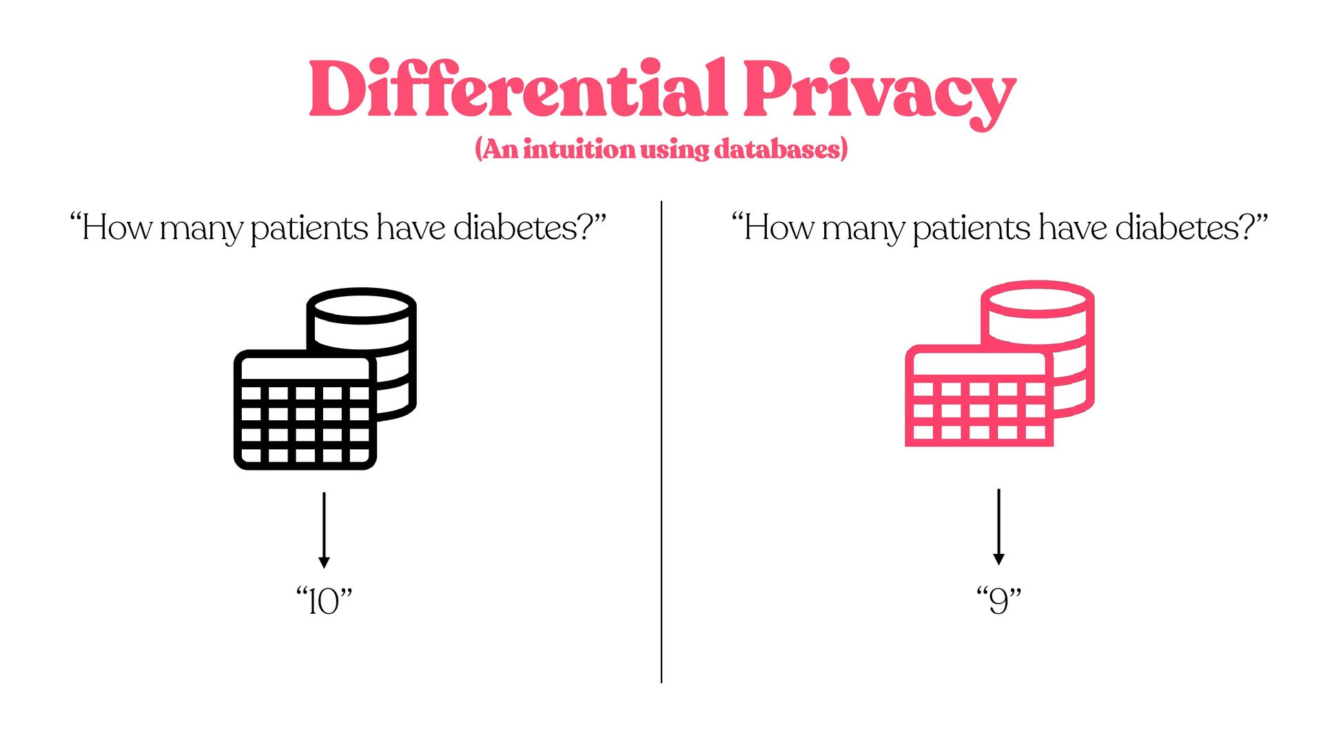
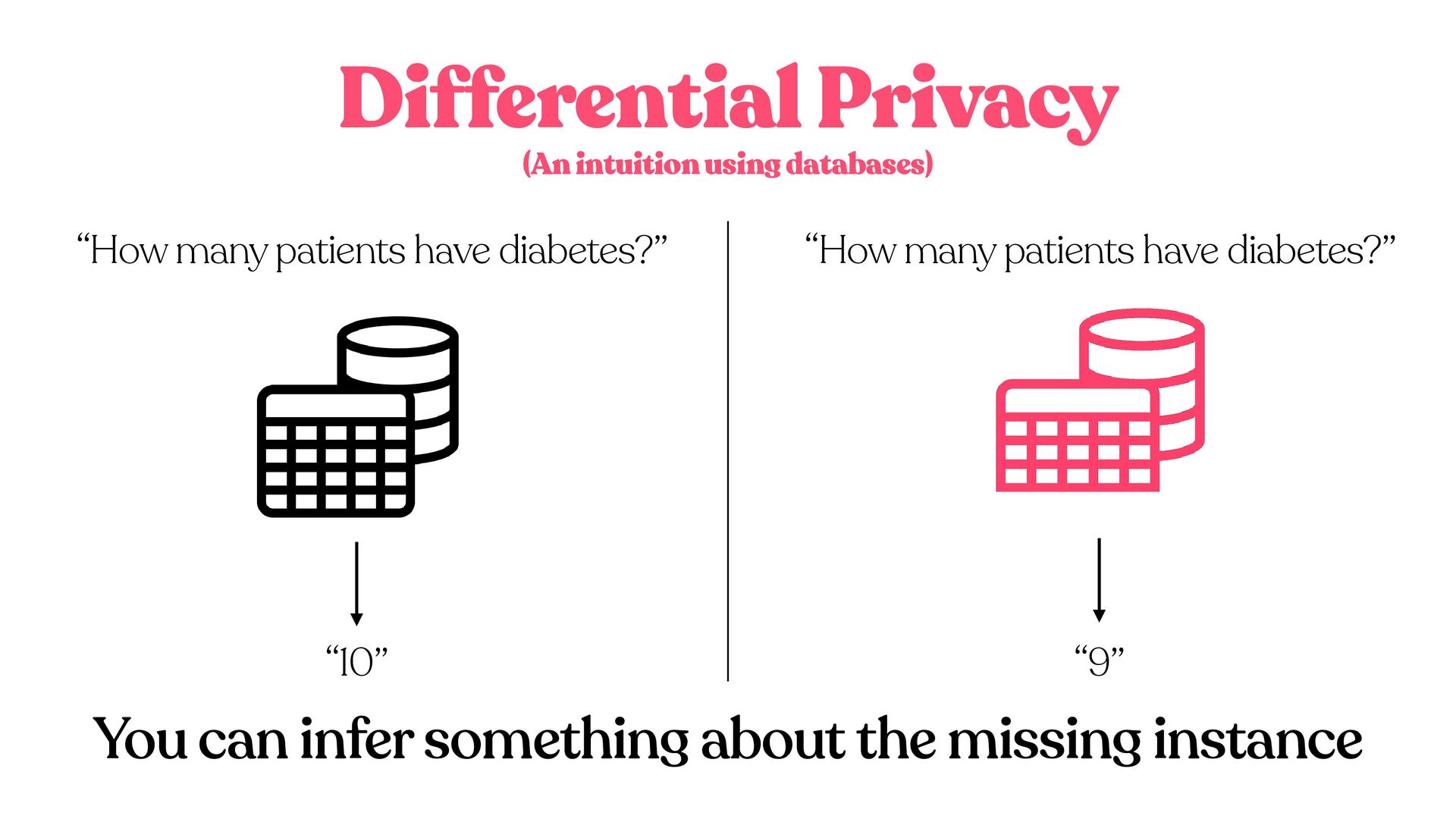
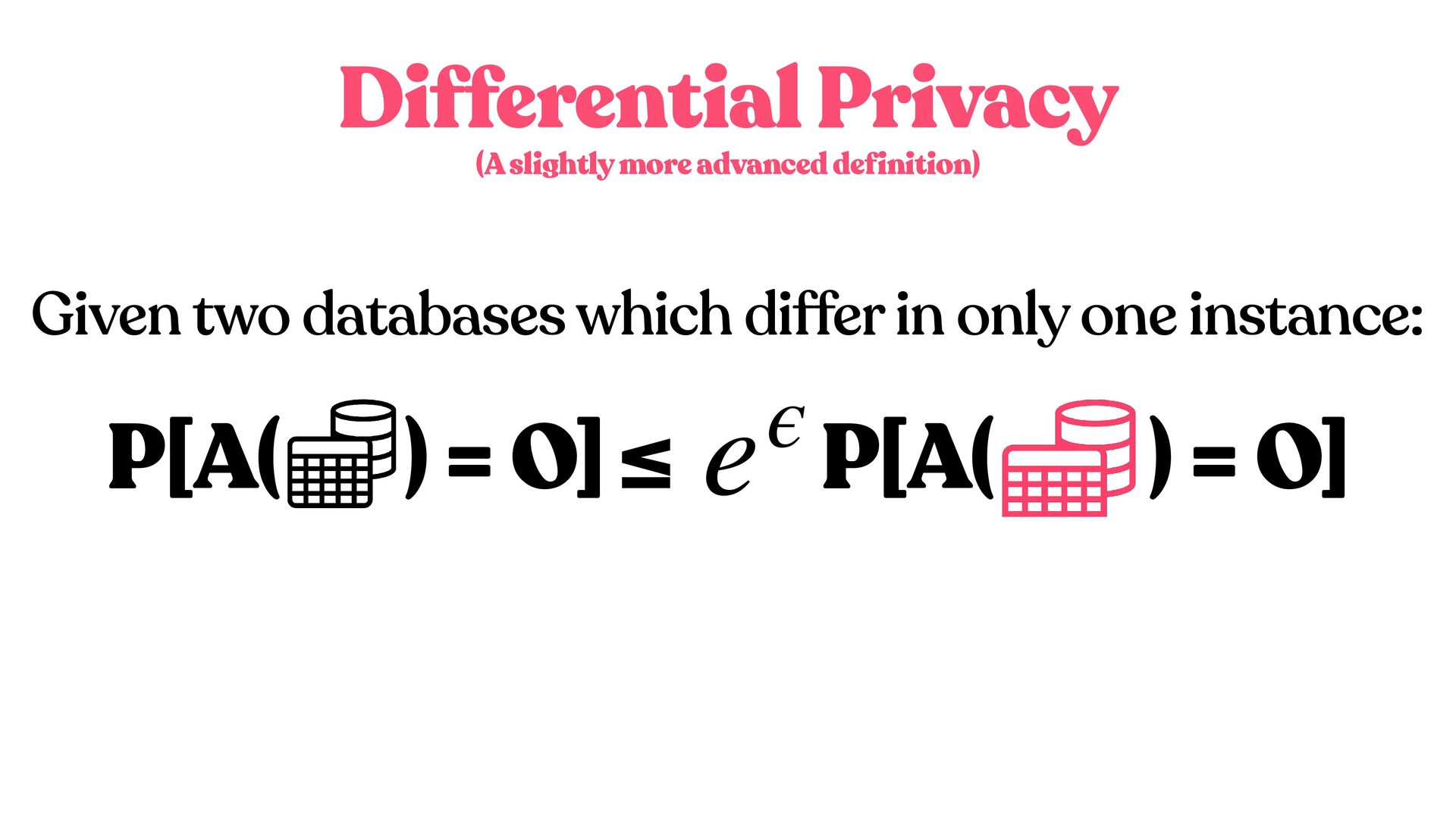
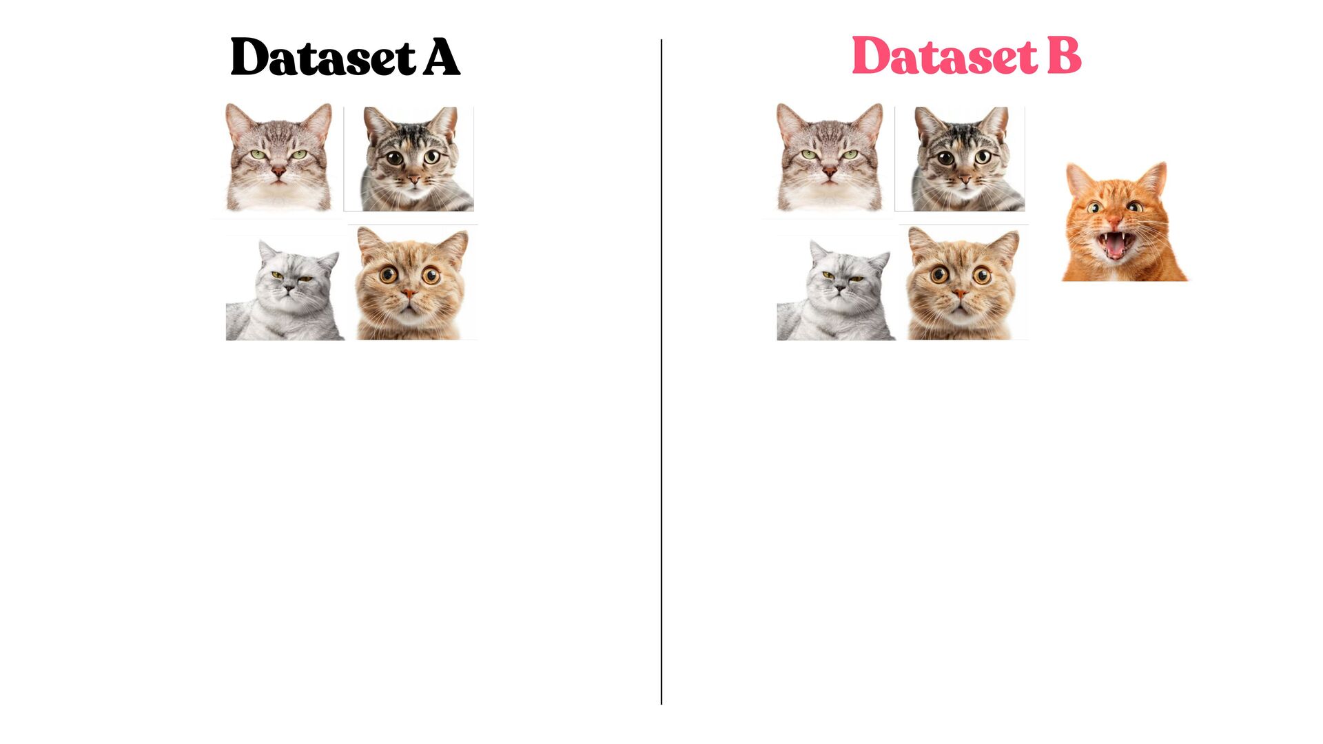
tells us how much these two probabilities are similar eϵ is called “privacy budget” and represents an upper bound on how much we can leak information ϵ How to interpret the ϵ Given two databases which differ in only one instance:
≤ P[A( ) = O] +δ eϵ The parameter quantifies the probability that something goes wrong. The algorithm will be differentially private with probability 1 -δ δ Given two databases which differ in only one instance:
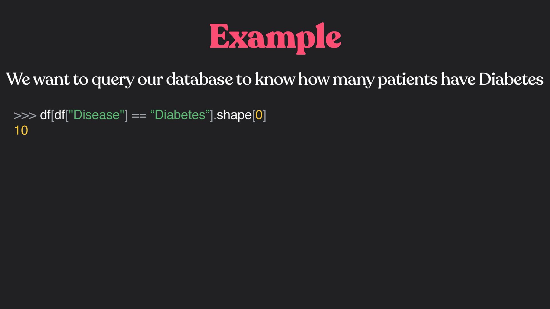
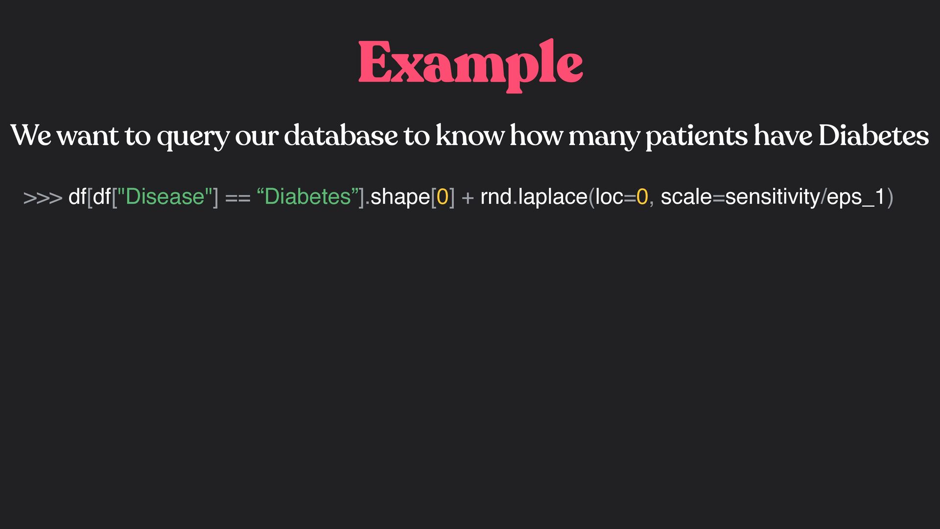
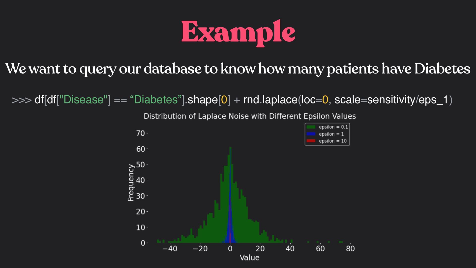
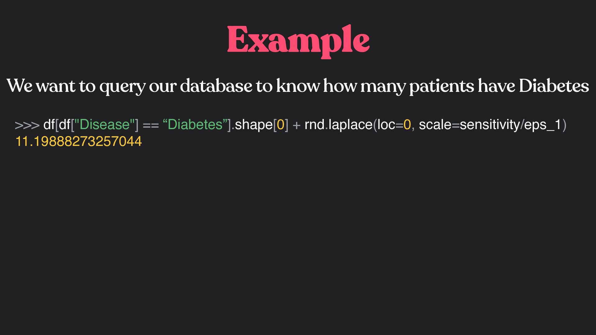
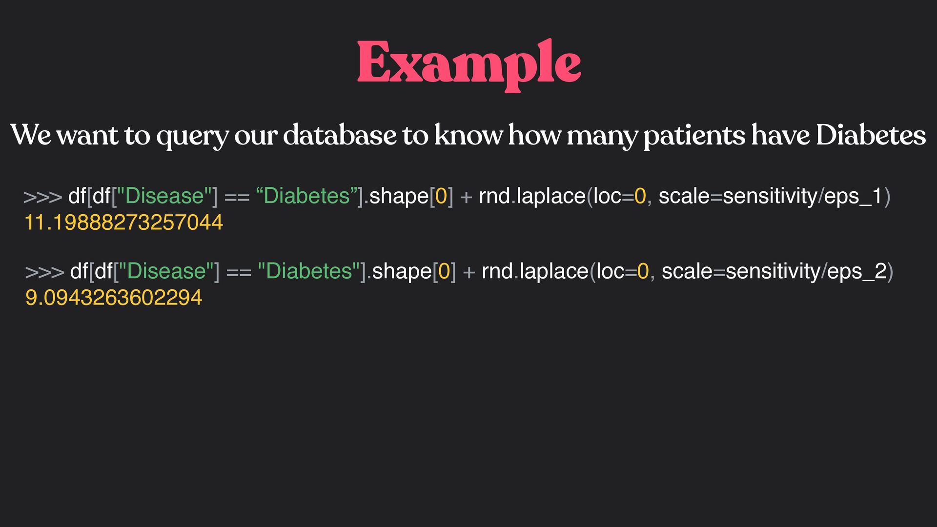
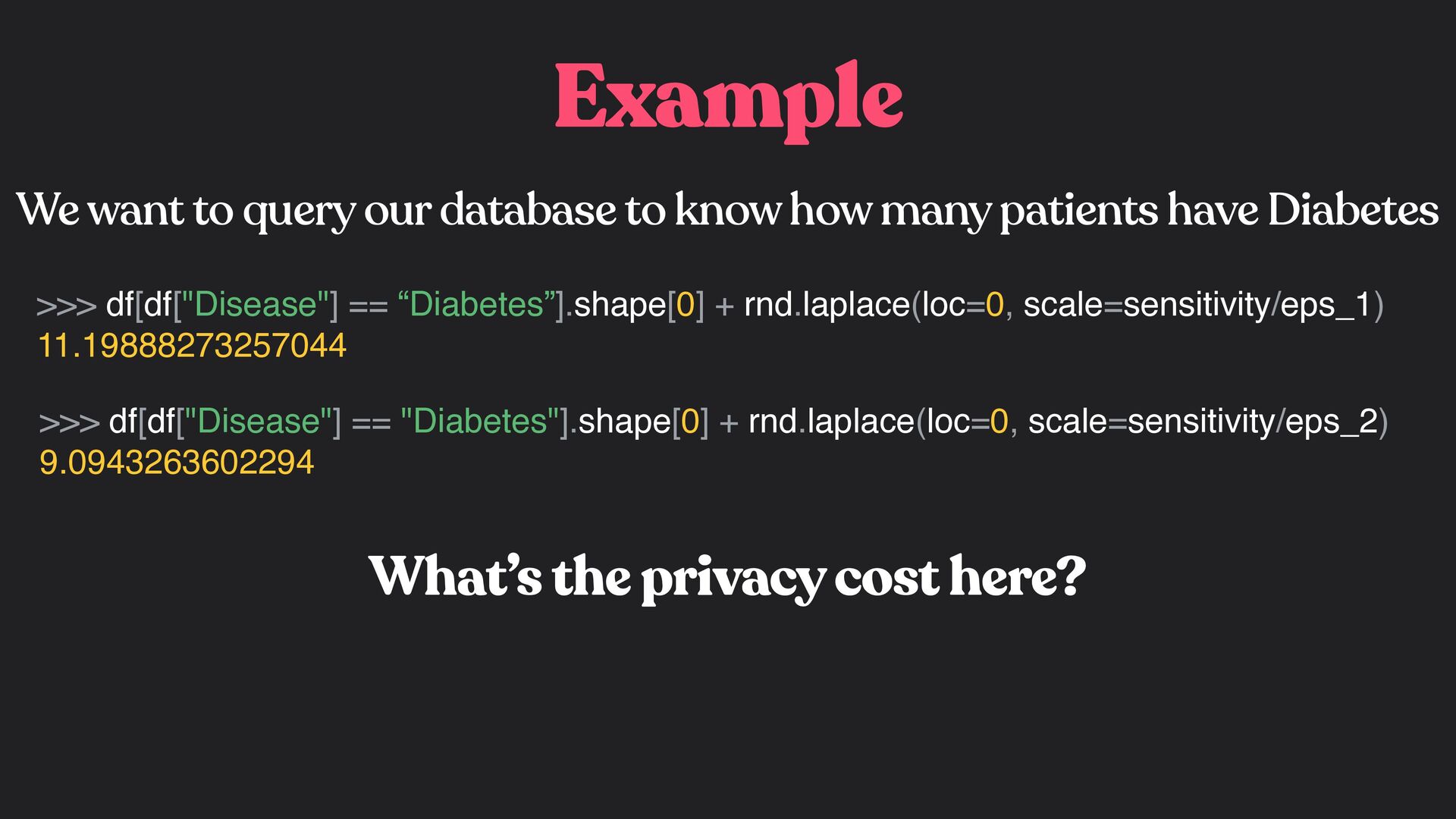
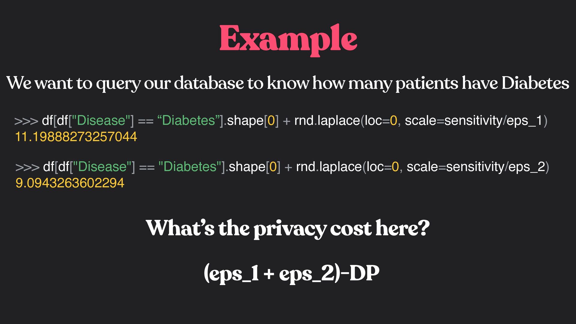
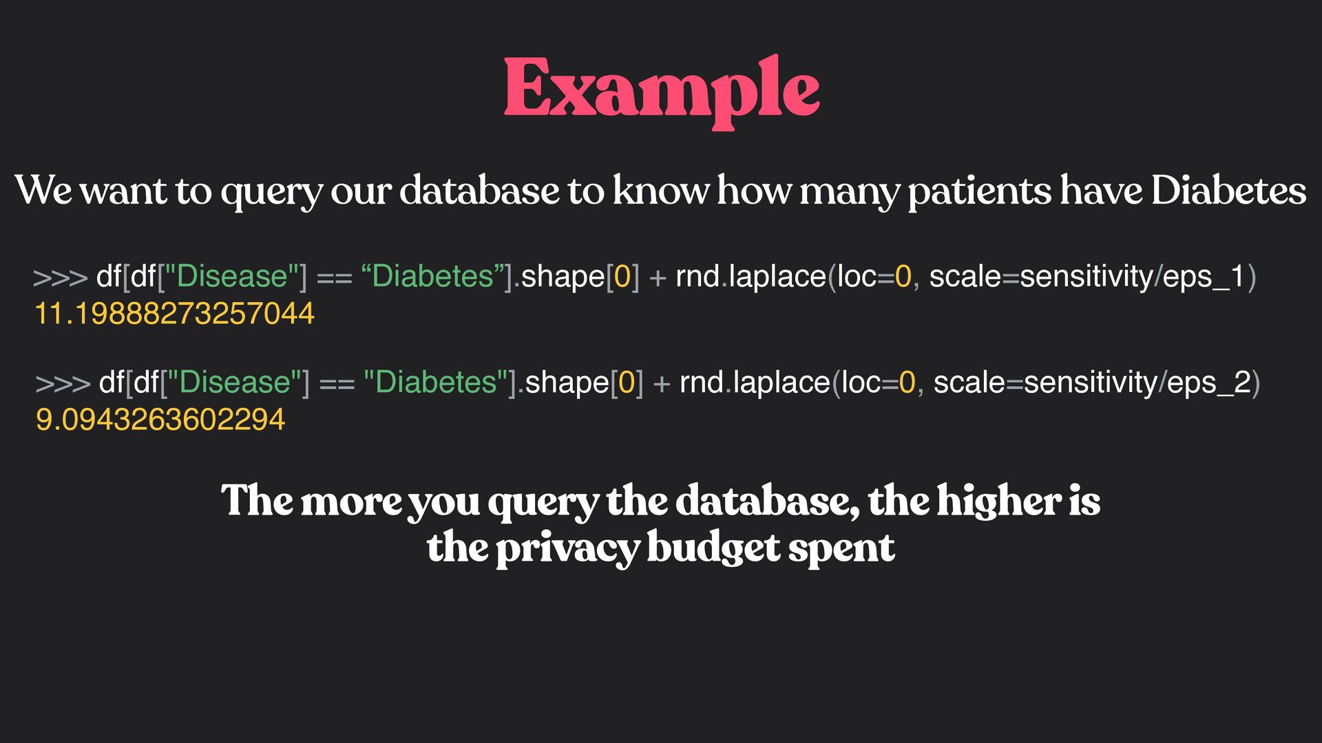
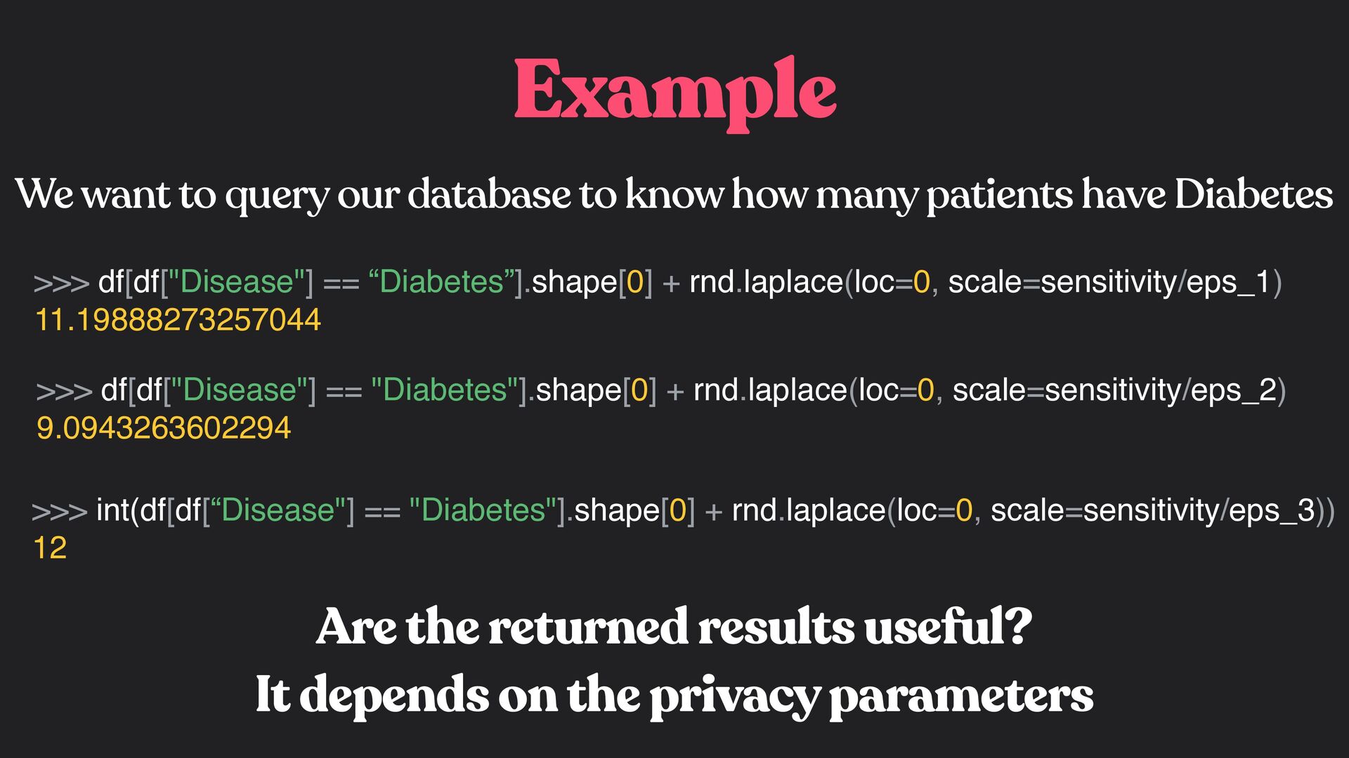
many patients have Diabetes >>> df[df["Disease"] == “Diabetes”].shape[0] + rnd.laplace(loc=0, scale=sensitivity/eps_1) 11.19888273257044 >>> df[df["Disease"] == "Diabetes"].shape[0] + rnd.laplace(loc=0, scale=sensitivity/eps_2) 9.0943263602294 The more you query the database, the higher is the privacy budget spent
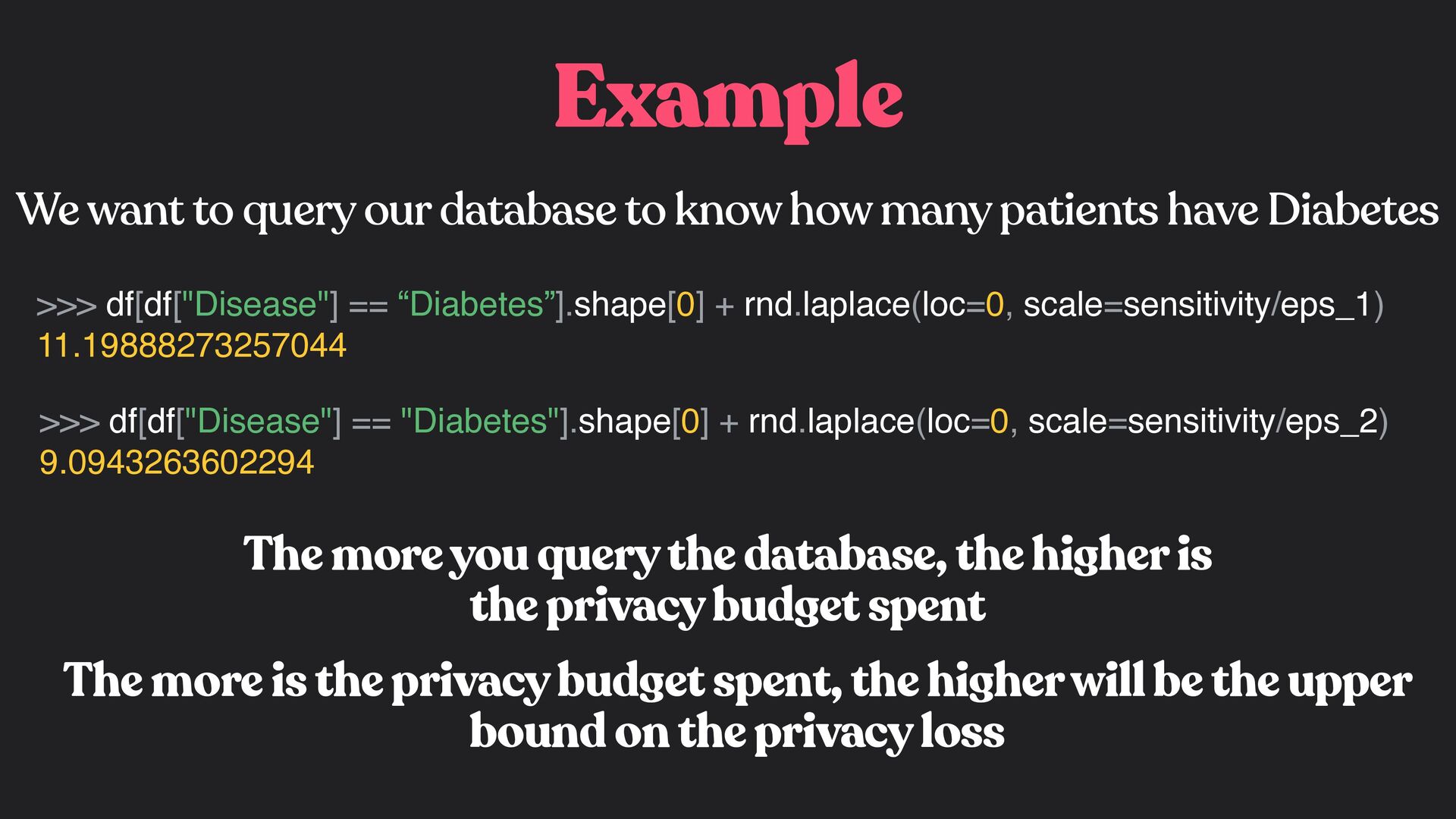
many patients have Diabetes >>> df[df["Disease"] == “Diabetes”].shape[0] + rnd.laplace(loc=0, scale=sensitivity/eps_1) 11.19888273257044 >>> df[df["Disease"] == "Diabetes"].shape[0] + rnd.laplace(loc=0, scale=sensitivity/eps_2) 9.0943263602294 The more you query the database, the higher is the privacy budget spent The more is the privacy budget spent, the higher will be the upper bound on the privacy loss
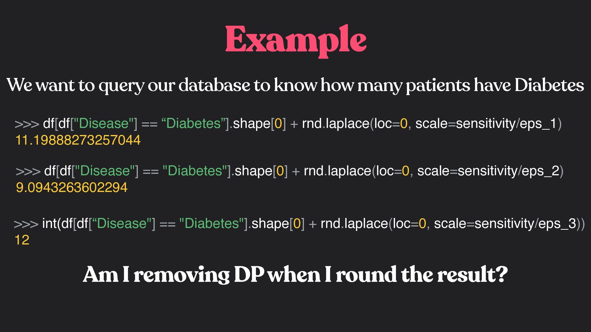
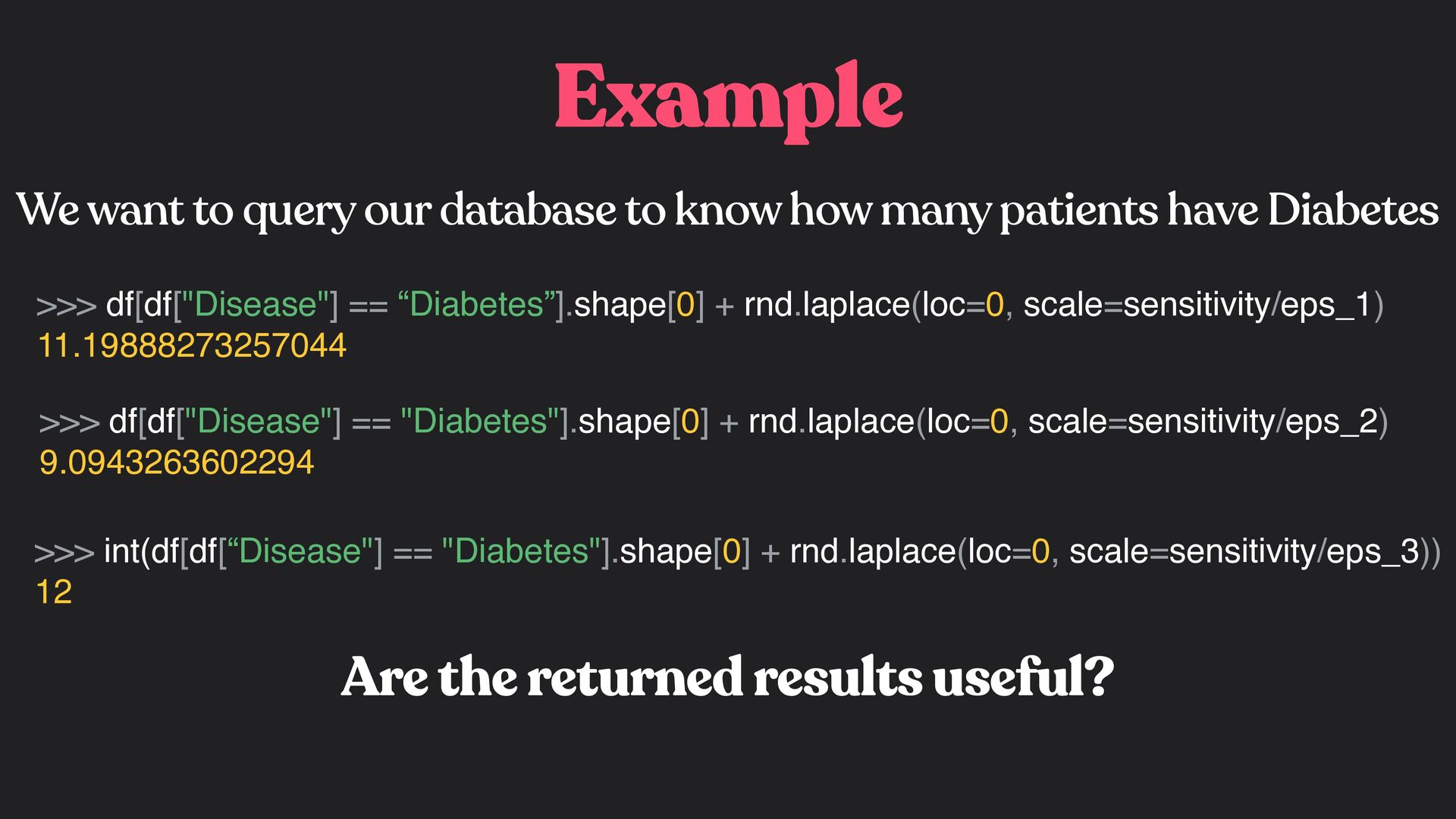
many patients have Diabetes >>> df[df["Disease"] == “Diabetes”].shape[0] + rnd.laplace(loc=0, scale=sensitivity/eps_1) 11.19888273257044 >>> df[df["Disease"] == "Diabetes"].shape[0] + rnd.laplace(loc=0, scale=sensitivity/eps_2) 9.0943263602294 >>> int(df[df[“Disease"] == "Diabetes"].shape[0] + rnd.laplace(loc=0, scale=sensitivity/eps_3)) 12 Are the returned results useful? It depends on the privacy parameters
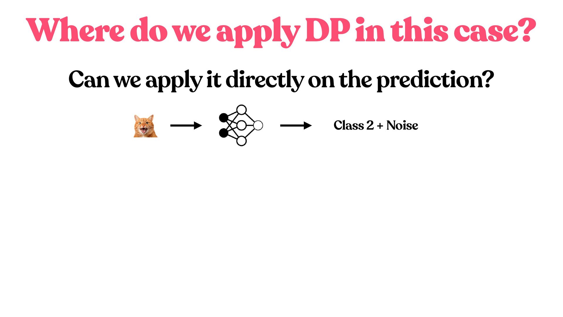
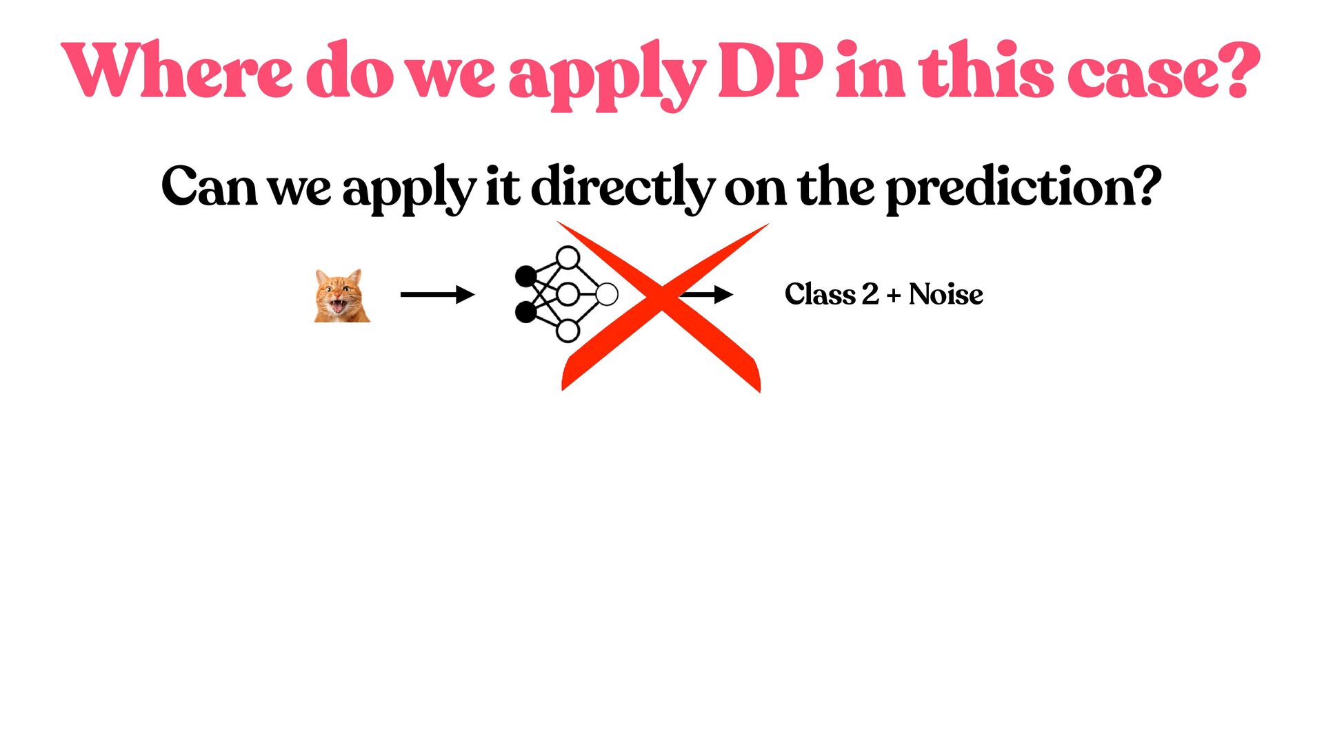
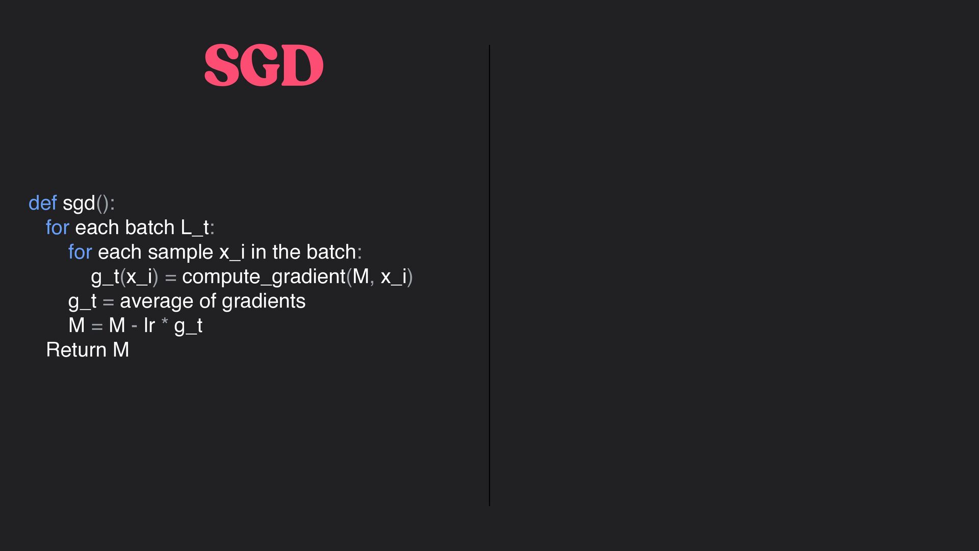
to apply it DURING the training The privacy budget will be spent during the training Once trained, we can query the model without additional privacy cost
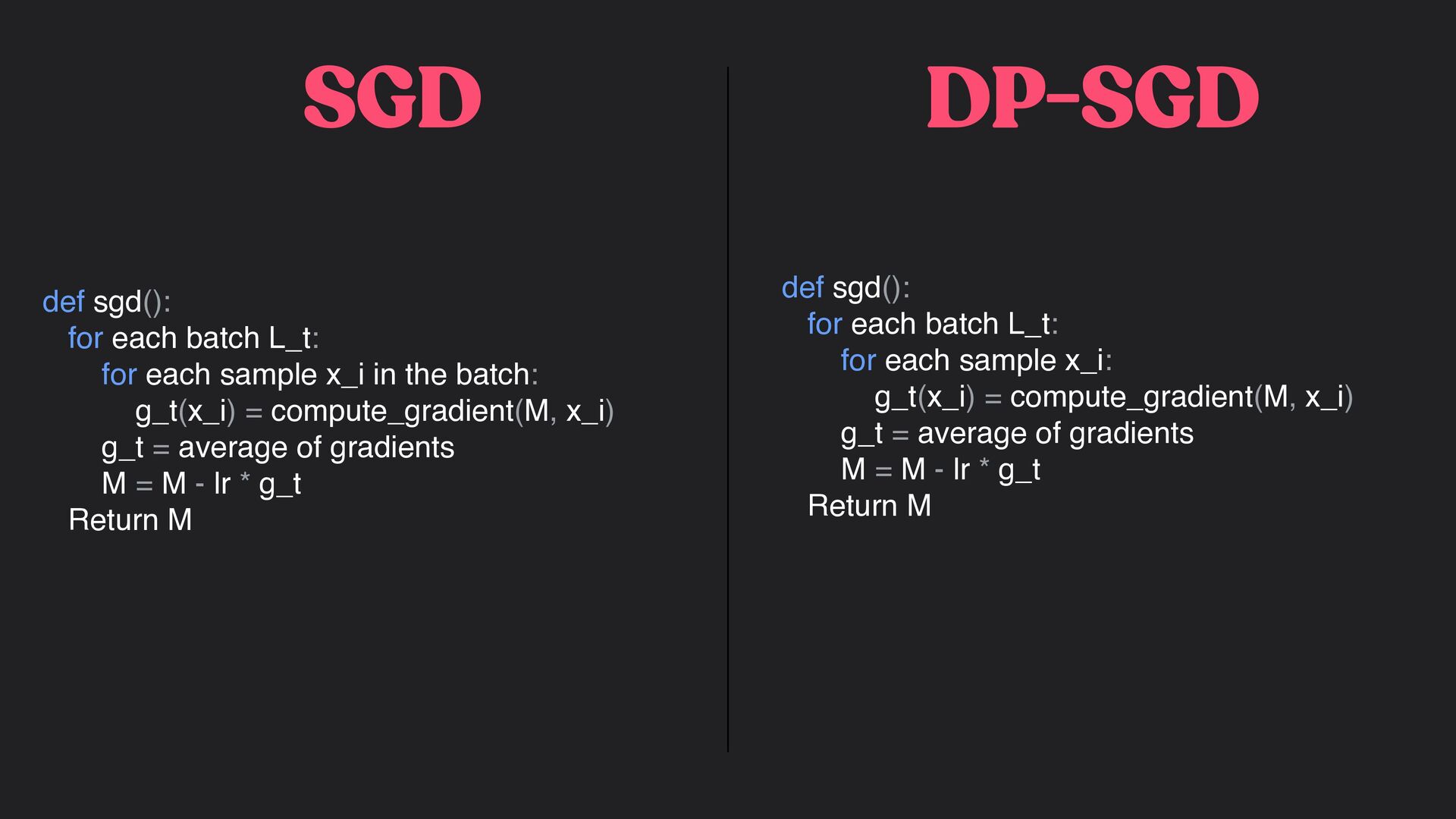
sample x_i in the batch: g_t(x_i) = compute_gradient(M, x_i) g_t = average of gradients M = M - lr * g_t Return M def sgd(): for each batch L_t: for each sample x_i: g_t(x_i) = compute_gradient(M, x_i) g_t = average of gradients M = M - lr * g_t Return M
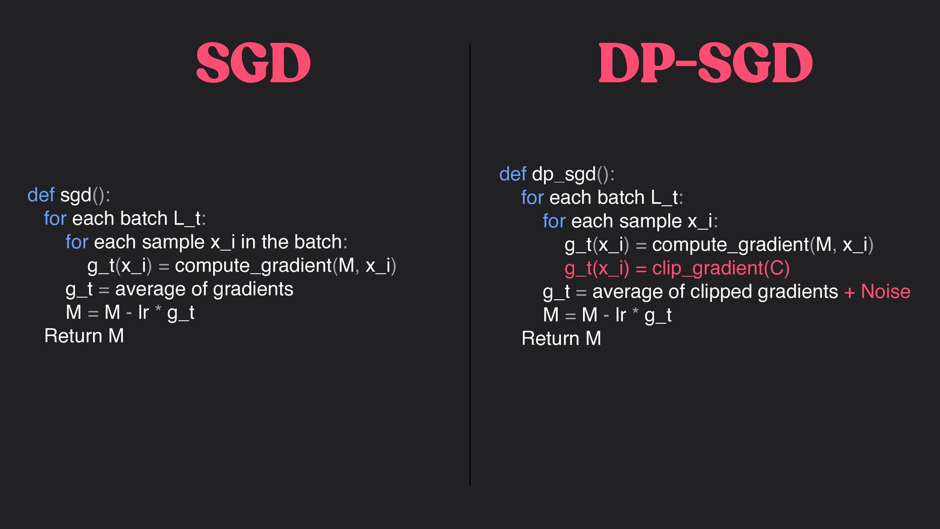
sample x_i: g_t(x_i) = compute_gradient(M, x_i) g_t(x_i) = clip_gradient(C) g_t = average of clipped gradients + Noise M = M - lr * g_t Return M def sgd(): for each batch L_t: for each sample x_i in the batch: g_t(x_i) = compute_gradient(M, x_i) g_t = average of gradients M = M - lr * g_t Return M
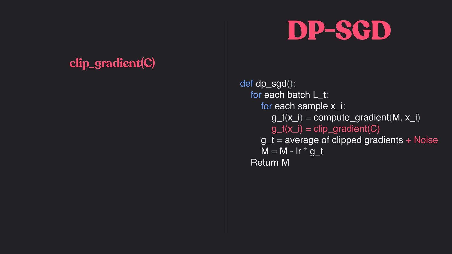
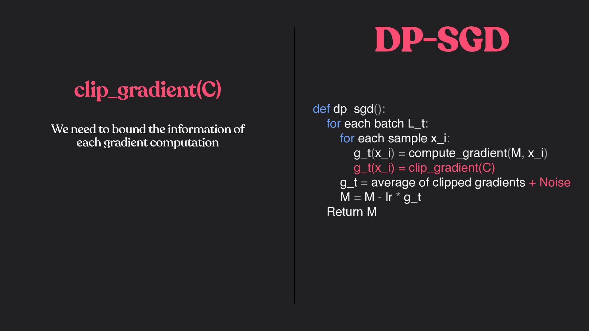
x_i: g_t(x_i) = compute_gradient(M, x_i) g_t(x_i) = clip_gradient(C) g_t = average of clipped gradients + Noise M = M - lr * g_t Return M clip_gradient(C)
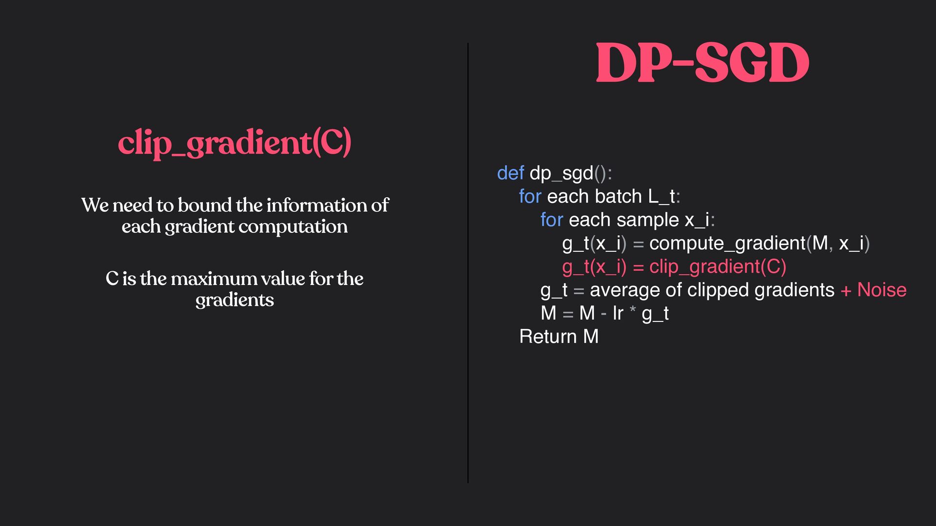
x_i: g_t(x_i) = compute_gradient(M, x_i) g_t(x_i) = clip_gradient(C) g_t = average of clipped gradients + Noise M = M - lr * g_t Return M clip_gradient(C) We need to bound the information of each gradient computation
x_i: g_t(x_i) = compute_gradient(M, x_i) g_t(x_i) = clip_gradient(C) g_t = average of clipped gradients + Noise M = M - lr * g_t Return M clip_gradient(C) We need to bound the information of each gradient computation C is the maximum value for the gradients
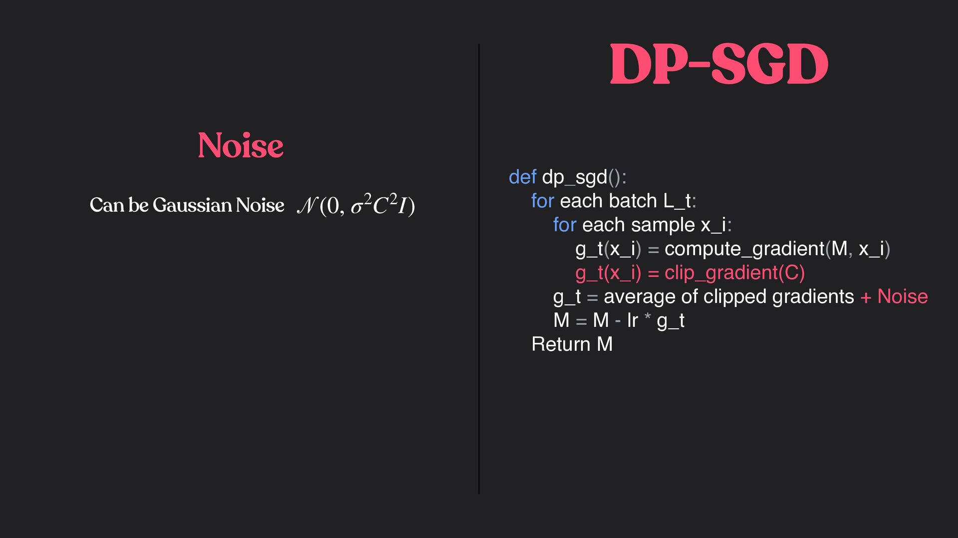
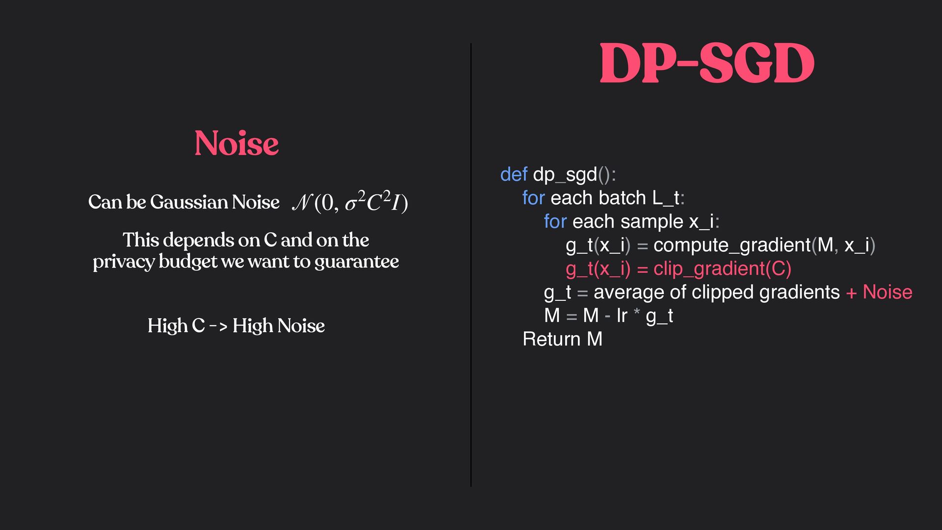
x_i: g_t(x_i) = compute_gradient(M, x_i) g_t(x_i) = clip_gradient(C) g_t = average of clipped gradients + Noise M = M - lr * g_t Return M 𝒩 (0, σ2C2I) Can be Gaussian Noise Noise
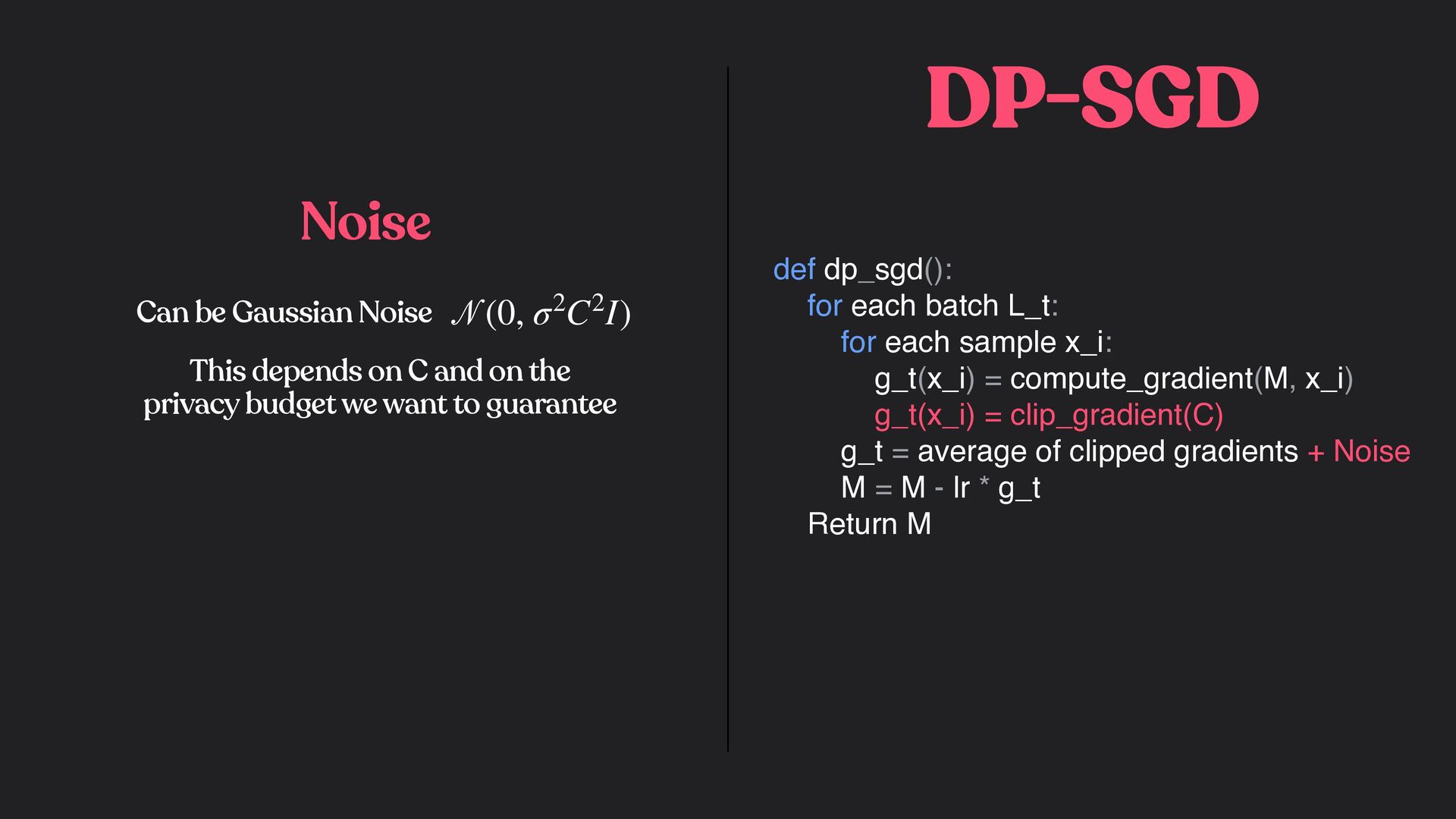
x_i: g_t(x_i) = compute_gradient(M, x_i) g_t(x_i) = clip_gradient(C) g_t = average of clipped gradients + Noise M = M - lr * g_t Return M 𝒩 (0, σ2C2I) Can be Gaussian Noise This depends on C and on the privacy budget we want to guarantee Noise
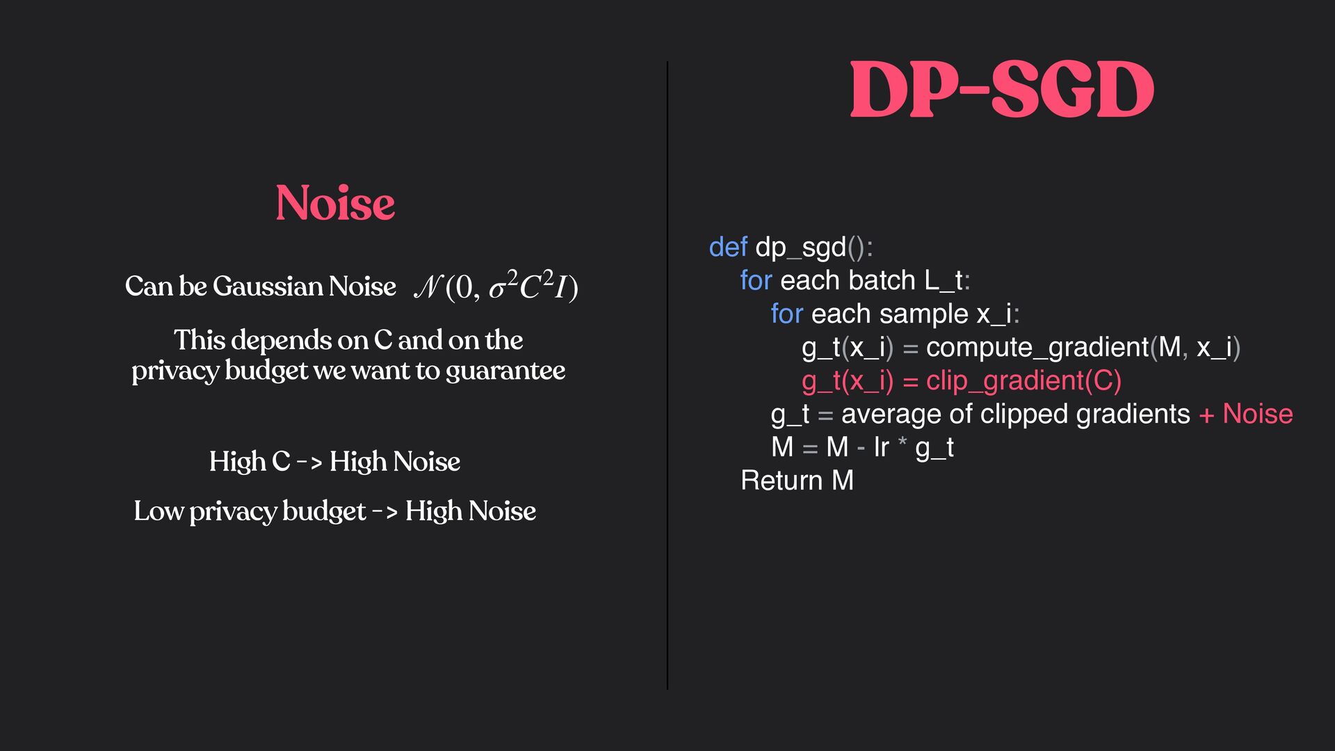
x_i: g_t(x_i) = compute_gradient(M, x_i) g_t(x_i) = clip_gradient(C) g_t = average of clipped gradients + Noise M = M - lr * g_t Return M 𝒩 (0, σ2C2I) Can be Gaussian Noise This depends on C and on the privacy budget we want to guarantee High C -> High Noise Noise
x_i: g_t(x_i) = compute_gradient(M, x_i) g_t(x_i) = clip_gradient(C) g_t = average of clipped gradients + Noise M = M - lr * g_t Return M 𝒩 (0, σ2C2I) Can be Gaussian Noise This depends on C and on the privacy budget we want to guarantee High C -> High Noise Low privacy budget -> High Noise Noise
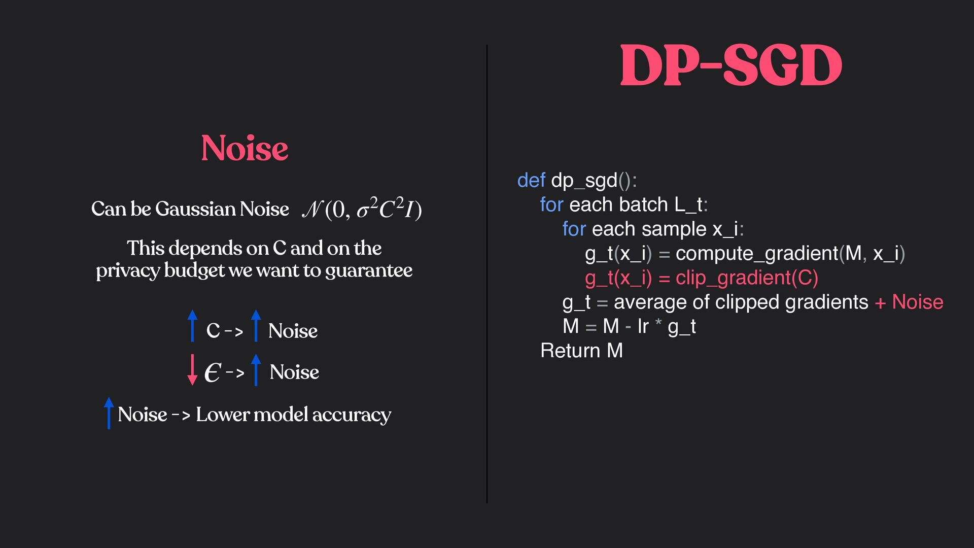
x_i: g_t(x_i) = compute_gradient(M, x_i) g_t(x_i) = clip_gradient(C) g_t = average of clipped gradients + Noise M = M - lr * g_t Return M 𝒩 (0, σ2C2I) Can be Gaussian Noise This depends on C and on the privacy budget we want to guarantee C -> Noise Noise -> Lower model accuracy Noise -> Noise ϵ
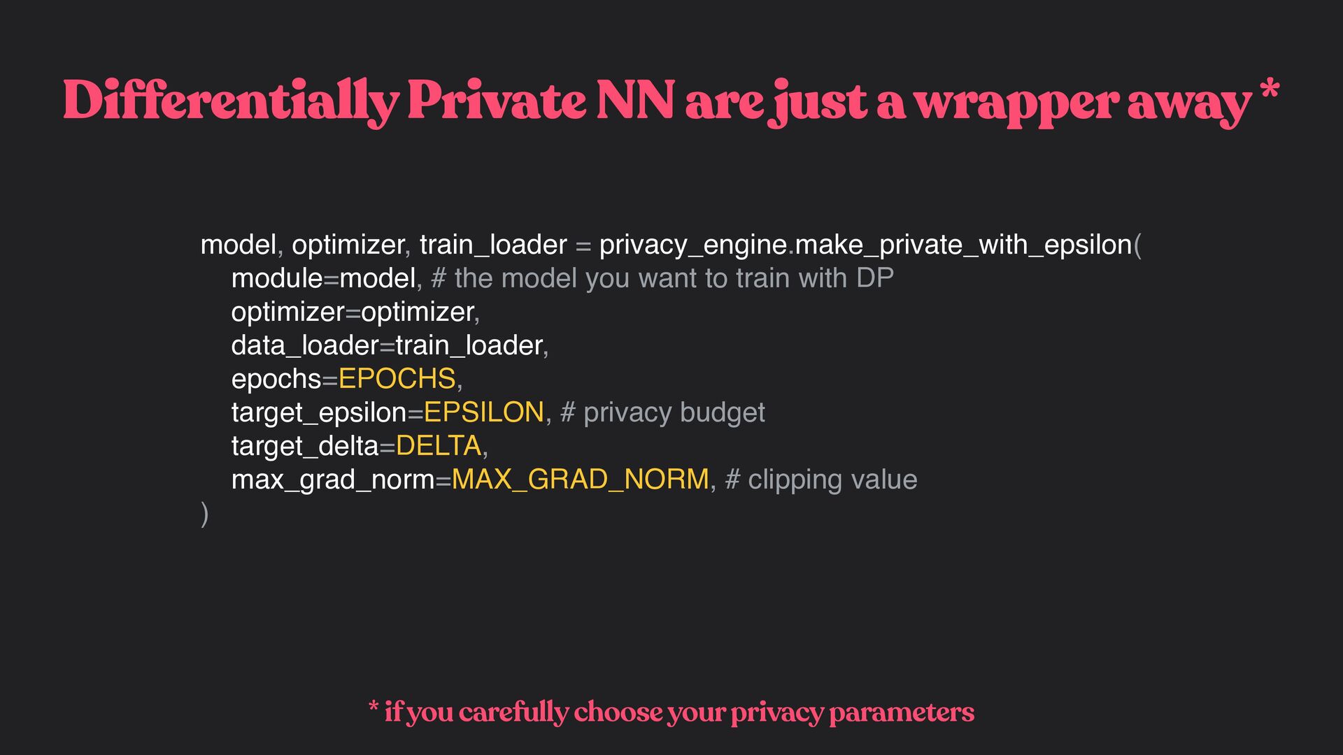
if you carefully choose your privacy parameters model, optimizer, train_loader = privacy_engine.make_private_with_epsilon( module=model, # the model you want to train with DP optimizer=optimizer, data_loader=train_loader, epochs=EPOCHS, target_epsilon=EPSILON, # privacy budget target_delta=DELTA, max_grad_norm=MAX_GRAD_NORM, # clipping value )
a low we will need to introduce a lot of noise during the training Choosing the is a tradeoff between the utility of the model and the privacy we want to guarantee ϵ ϵ
a low we will need to introduce a lot of noise during the training This will degrade the model performances! Choosing the is a tradeoff between the utility of the model and the privacy we want to guarantee ϵ ϵ
![P[A( ) = O] ≤ P[A( ) = O] eϵ](https://files.speakerdeck.com/presentations/2ede5ec390e34c6a881751301935ac50/slide_30.jpg)
![Differential Privacy (A more relaxed definition) P[A( ) = O]](https://files.speakerdeck.com/presentations/2ede5ec390e34c6a881751301935ac50/slide_31.jpg)
![Differential Privacy P[A( ) = ] ≤ P[A( ) =](https://files.speakerdeck.com/presentations/2ede5ec390e34c6a881751301935ac50/slide_48.jpg)
![Differential Privacy P[A( ) = ] ≤ P[A( ) =](https://files.speakerdeck.com/presentations/2ede5ec390e34c6a881751301935ac50/slide_49.jpg)