The Unconventional Introduction to Deep Learning @ PyData Florence

If you talk (a lot) about Deep Learning, sooner or later, it inevitbly happens that you're asked
to explain what actually **Deep Learning** means, and what's all the fuss about it.

Indeed, answering this question in a proper way, may vary (and it has to) depending on
the kind of audience you've been talking to.

If you are talking to machine learning experts, you have to concentrate on what _deep_
means for the multiple learning models you can come up with.
Most importarly, you have to be very convincing about the performance of a deep learning model
against more standard and robust Random Forest or Support Vector Machine.

If your audience is made up of engineers, it is a completely different story.
Engineers don't give a damn.. are definitely more interested in how
implementing Artificial Neural Networks (ANN) in the most productive way, rather than
really understanding what are the implications of different *activations* and *optimizers*.

Eventually, if your audience is made up of data scientists - intended as the perfect mixture of the
previous two categories - according to
[Drew Conway](http://drewconway.com/zia/2013/3/26/the-data-science-venn-diagram) -
they are more or less interested in both the two aspects.

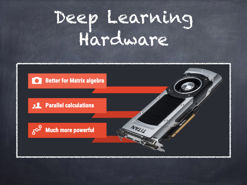
The other way, that is the _unconventional way_, to talk about Deep Learning,
is from the perspective of the computational model it requires to be properly effective.
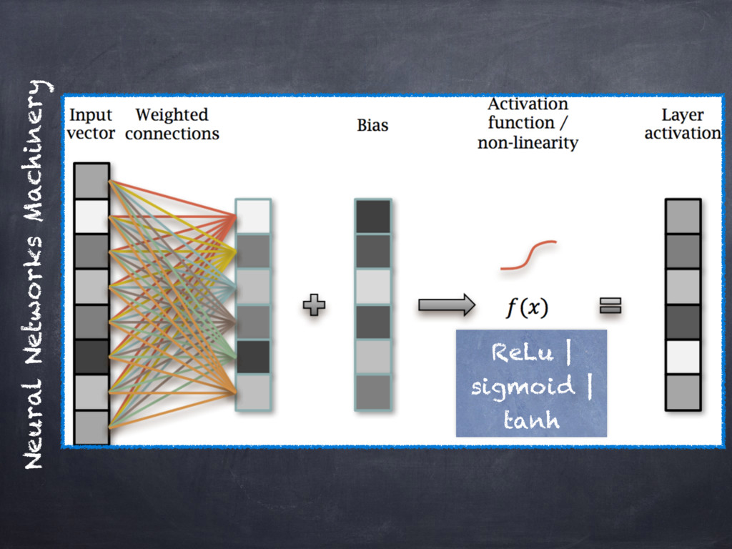
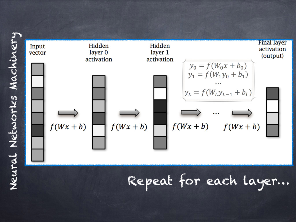
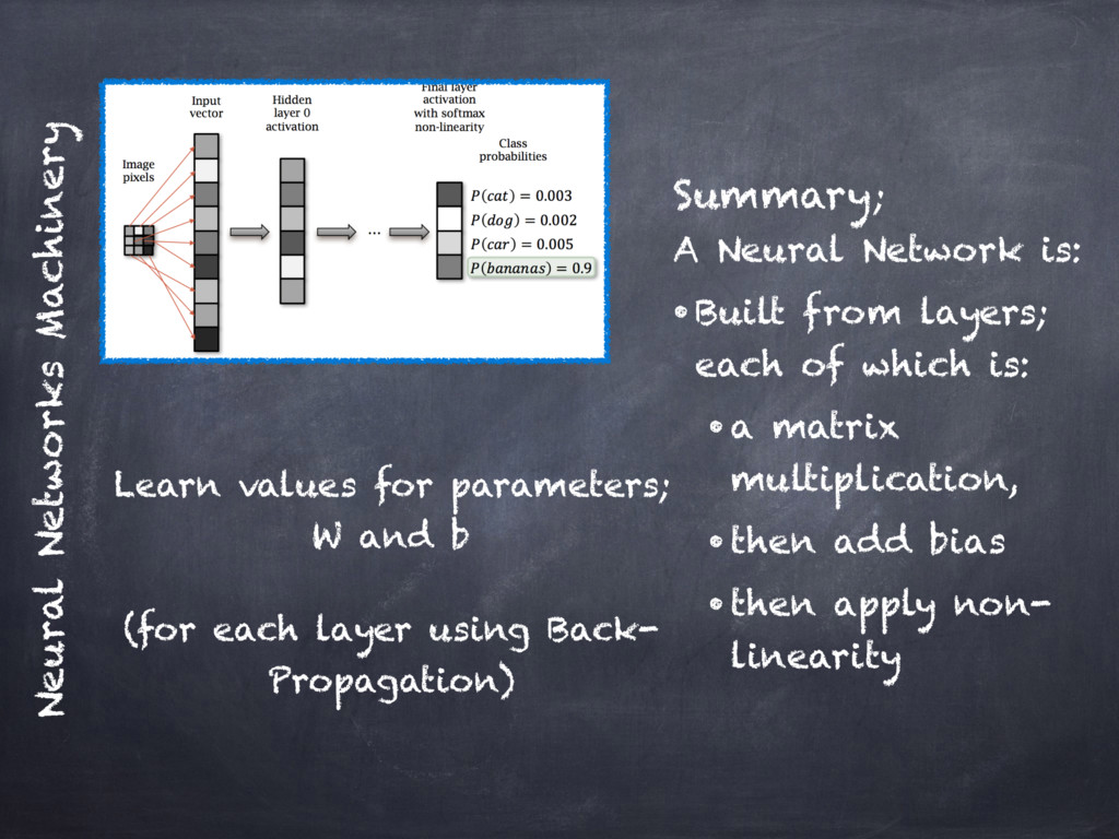
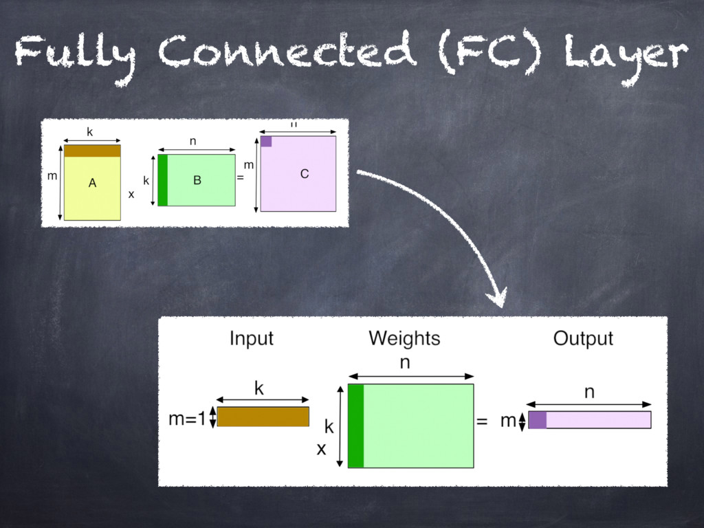
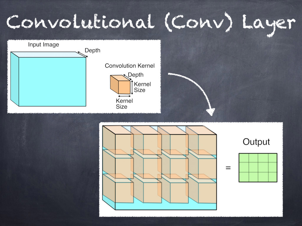
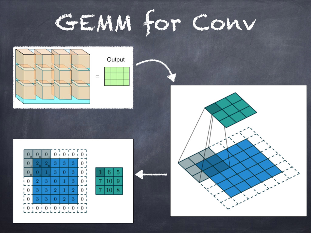
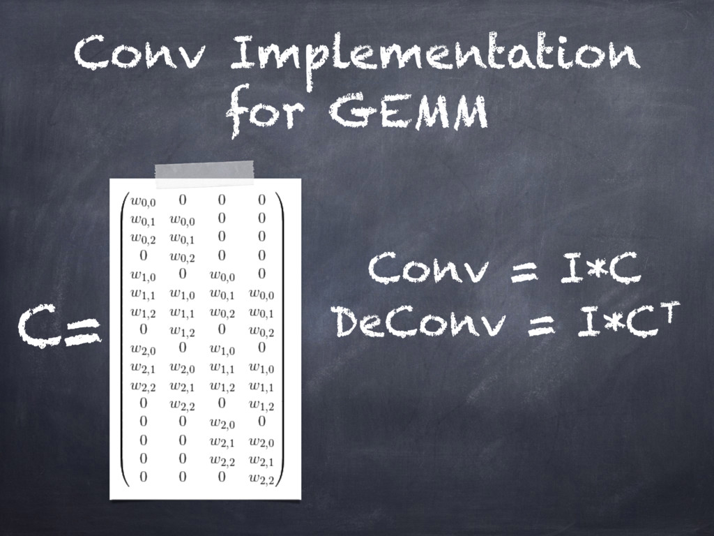
Therefore, you may want to talk about ANN in terms of matrix multiplications algorithms,
parallel execution models, and GPU computing.
And this is **exactly** the perspecitve I intend to pursue in this talk.

This talk is for PyData scientists who are interested in understanding Deep Learning models
from the unconventional perspective of the GPUs.
Experienced engineers may likely benefit from this talk as well, learning how they can make their
models run fast(er).
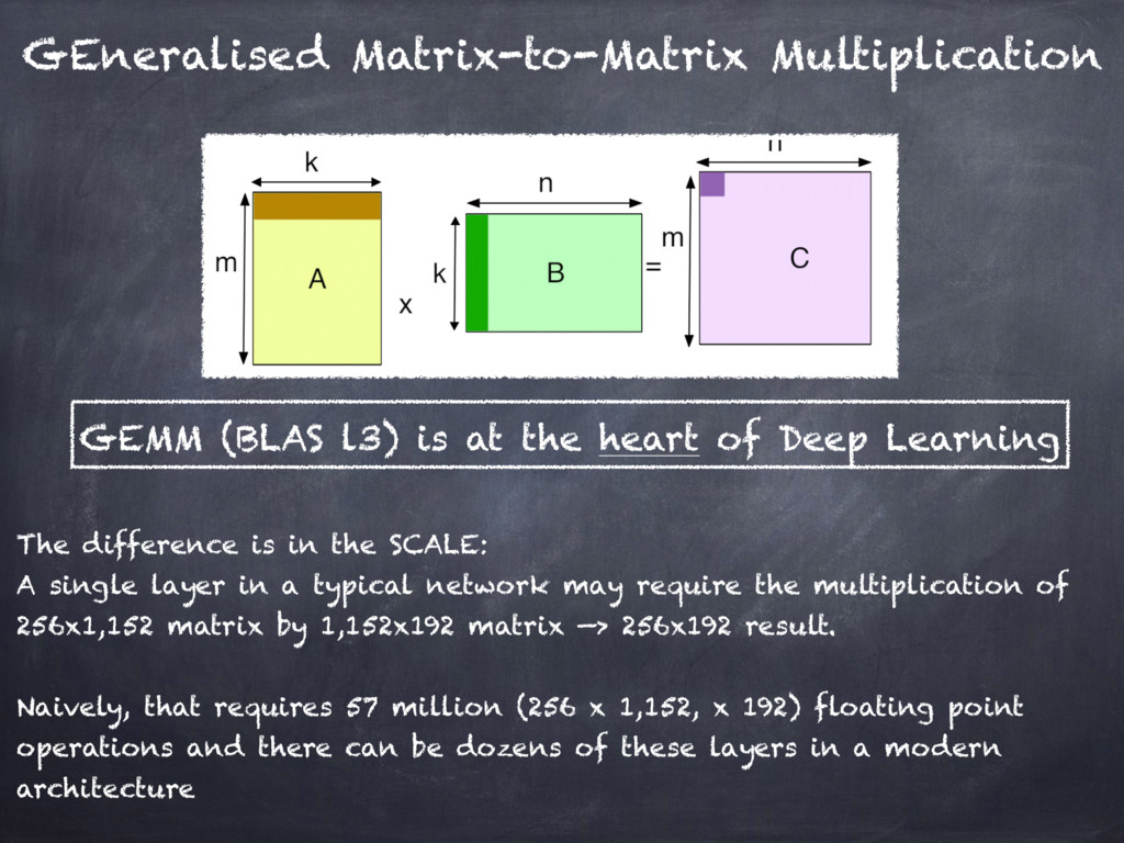
ANNs will be presented in terms of
_Accelerated Kernel Matrix Multiplication_ and the `gem[m|v]` BLAS library.
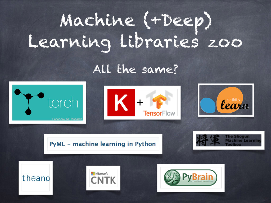
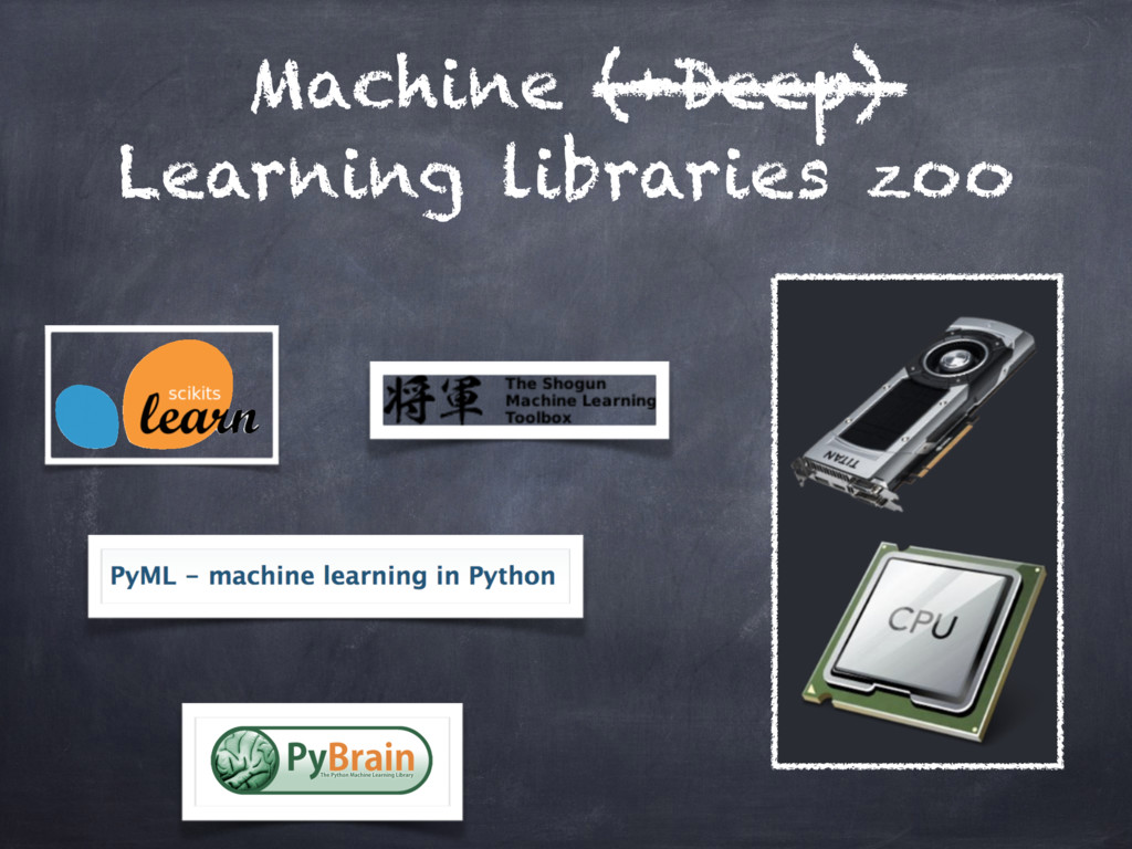
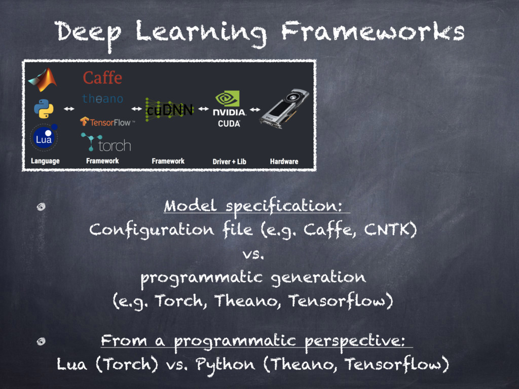
Different libraries and tools from the Python ecosystem will be presented (e.g. `numba`, `theano`, `tensorflow`).

Transcript

1. Deep Learning in Python The Unconventional Introduction Data Scientist and Researcher Fondazione Bruno Kessler (FBK)
 Trento, Italy Valerio Maggio @leriomaggio
4. Hint:
 Doctor Who?
5. Quite Common Deep Learning Intro
7. A multi-layer feed-forward neural network that starts w/ an input layer fully connected, which is followed by multiple hidden layer of non-linear transformation Neural Network Introduction
9. Neural Networks Machinery
10. Neural Networks Machinery ReLu | sigmoid | tanh
11. Neural Networks Machinery Repeat for each layer…
12. Neural Networks Machinery Image Classification Task
13. Neural Networks Machinery Summary; 
 A Neural Network is: • Built from layers; each of which is: • a matrix multiplication, • then add bias • then apply non- linearity Learn values for parameters; W and b (for each layer using Back- Propagation)
15. Deep Networks
16. Deep Networks
18. Deep Learning is quite like the Tardis…
19. Deeply Wobbly, Timey Wimey… stuff
20. So, what about Python?
21. Machine (+Deep) Learning libraries zoo All the same?
22. Machine (+Deep) Learning libraries zoo
23. Deep Learning Hardware
24. VGG16: 
 Fully Convolutional Neural Network (FCNN) Vanilla VGG16 VGG16
25. Source: Learning Semantic Image Representations at a Large Scale
26. GEneralised Matrix-to-Matrix Multiplication GEMM (BLAS l3) is at the heart of Deep Learning The difference is in the SCALE:
 A single layer in a typical network may require the multiplication of 256x1,152 matrix by 1,152x192 matrix —> 256x192 result. 
 Naively, that requires 57 million (256 x 1,152, x 192) floating point operations and there can be dozens of these layers in a modern architecture
27. Fully Connected (FC) Layer
28. Convolutional (Conv) Layer
29. GEMM for Conv
30. Conv Implementation for GEMM C= Conv = I*C DeConv = I*CT
31. Deep Learning Frameworks
32. Deep Learning Frameworks Model specification: 
 Configuration file (e.g. Caffe, CNTK) 
 vs. 
 programmatic generation 
 (e.g. Torch, Theano, Tensorflow) From a programmatic perspective: 
 Lua (Torch) vs. Python (Theano, Tensorflow)
33. import tensorflow as tf vs. import theano as th Theano is a deep learning library with python wrapper (inspiration for tensorflow) Tensorflow is a deep learning library recently open sourced by Google th ~= tf: tf has better support for distributed systems
34. What does 
 tensorflow provides? TensorFlow provides primitives for defining functions on tensors and automatically computing their derivatives
35. Tensor?
36. Tensor?
37. Tensor? An intuitive way to represent a tensor is a
 multidimensional array
38. numpy vs tensorflow
39. tf requires explicit evaluation In [1]: import numpy as np In [2]: import tensorflow as tf In [3]: a = np.zeros((2,2) In [4]: ta = tf.zeros((2,2)) In [5]: print(a) [[ 0. 0.] [ 0. 0.]] In[6]: print(ta) Tensor("zeros_1:0", shape=(2, 2), dtype=float32) In[7]: print(ta.eval()) [[ 0. 0.] [ 0. 0.]]
40. tf.Graph (IDEA) A Machine Learning application is the result of the repeated computation of complex mathematical expressions, thus we could describe this computation by using a Data Flow Graph Data Flow Graph: each Node represents the instance of a mathematical operation:
 multiply, add, divide each Edge is a multi-dimensional data set (tensors) on which the operations are performed.
41. tf.Graph Node: instantiation of an operation w/ 
 inputs (>= 2), outputs >= 0. Data Edges: 
 carriers tensors, where an output of one operation (from one node) becomes the input for another operation. Dependency Edges: 
 control dependency between two nodes (i.e. "happens before" relationship). Before and after graph transformation for partial execution
42. Logistic Regression
43. source: https:/ /github.com/tensorflow/fold tf.Graph w/ multi-layers
44. Logistic Neuron
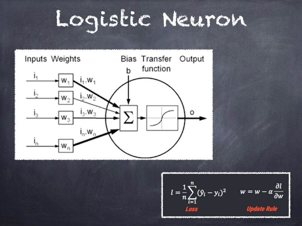
45. Logistic Neuron In [1]: import tensorflow as tf In [2]: # tf Graph Input x = tf.placeholder("float", [None, 784]) y = tf.placeholder("float", [None, 10])
 In [3]: # Set model weights W = tf.Variable(tf.zeros([784, 10])) b = tf.Variable(tf.zeros([10]))
 In [4]: # Construct model activation = tf.nn.softmax(tf.matmul(x, W) + b) # Softmax
 In [5]: # Minimize error using cross entropy cross_entropy = y*tf.log(activation) cost = tf.reduce_mean(-tf.reduce_sum(cross_entropy,
 reduction_indices=1)) Repeat this for each layer you want to add
46. Logistic Neuron In [6]: learning_rate = 0.01 In [7]: # Set the Optimizer
 optimizer = tf.train.GradientDescentOptimizer(learning_rate).minimize(cost) In [9]: # Initializing the variables init = tf.global_variable_initializers() In[10]: for epoch in range(training_epochs): avg_cost = 0. total_batch = int(mnist.train.num_examples/batch_size) # Loop over all batches for i in range(total_batch): batch_xs, batch_ys = mnist.train.next_batch(batch_size) # Fit training using batch data sess.run(optimizer, feed_dict={x: batch_xs, y: batch_ys}) # Compute average loss avg_cost += sess.run(cost, 
 feed_dict={x: batch_xs, y: batch_ys}) / total_batch
47. Deep Learning: the Keras way @pydatait @pycon8
48. Thank you! @leriomaggio