Machine Learning model evaluation and assessment class - as part of the MSc in Medical Statistics and Health Data Science, University of Bristol (2023)
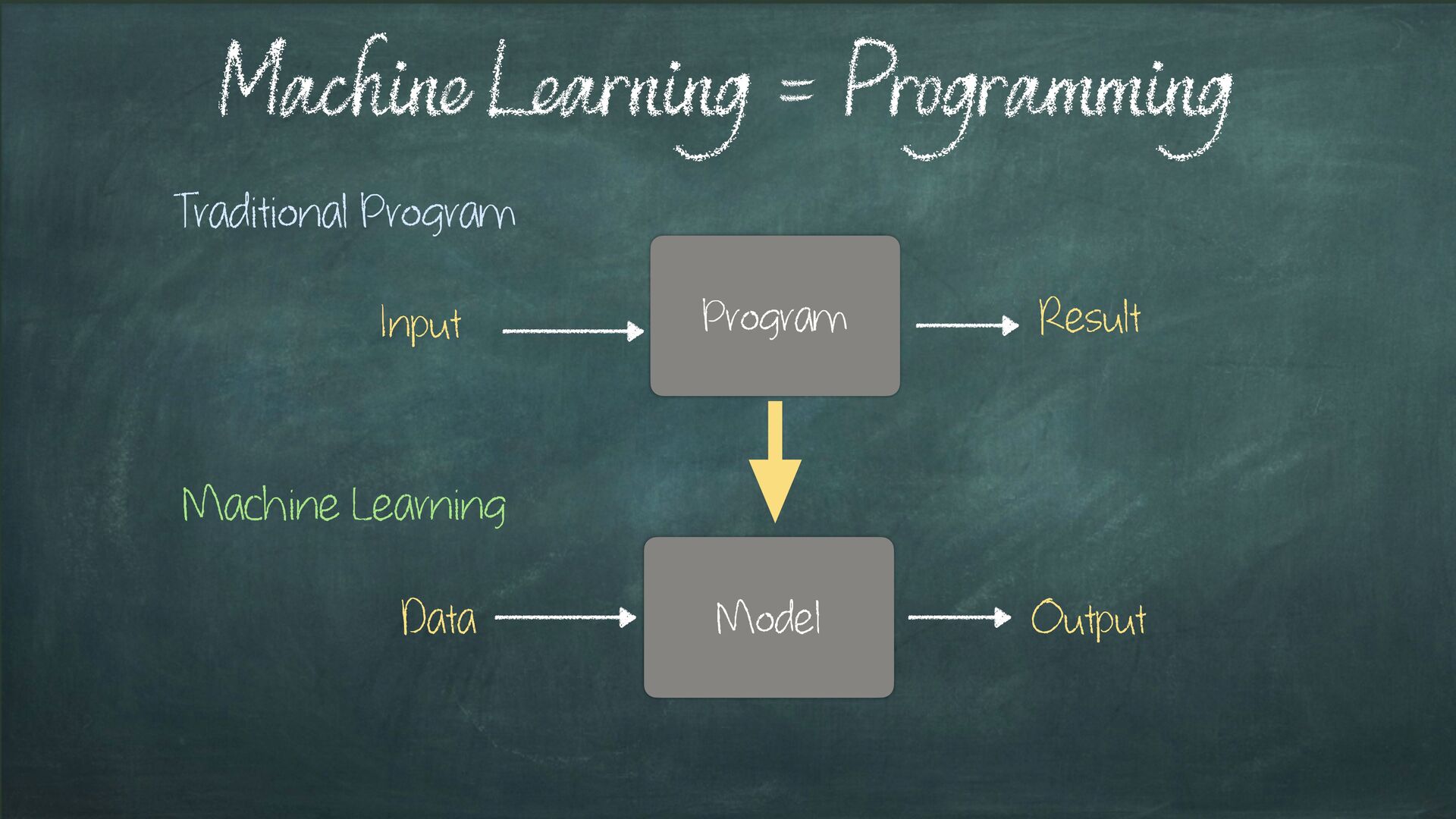
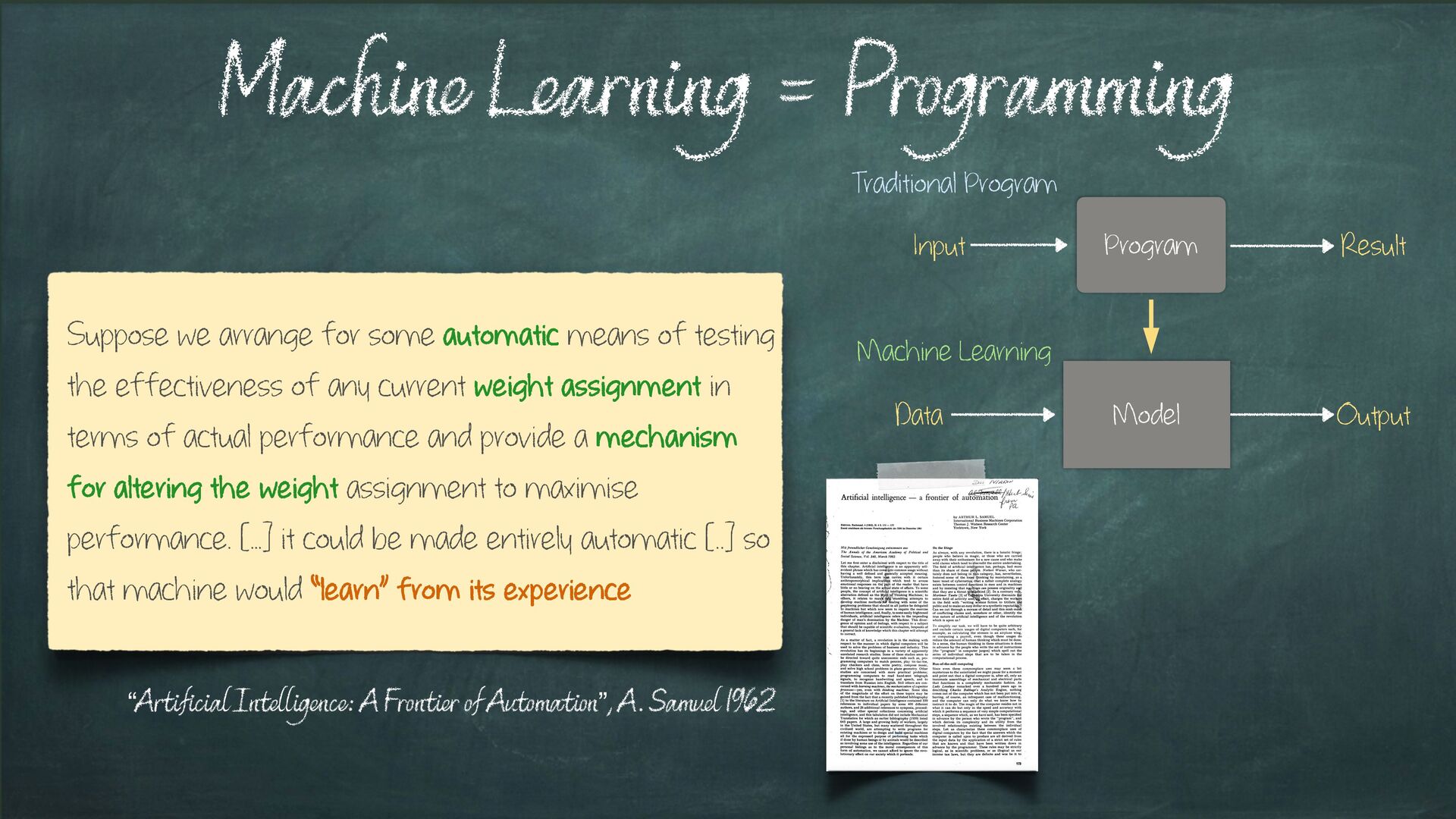
A. Samuel 1962 Suppose we arrange for some automatic means of testing the effectiveness of any current weight assignment in terms of actual performance and provide a mechanism for altering the weight assignment to maximise performance. […] it could be made entirely automatic [..] so that machine would “learn” from its experience Data Model Output Input Program Result Traditional Program Machine Learning
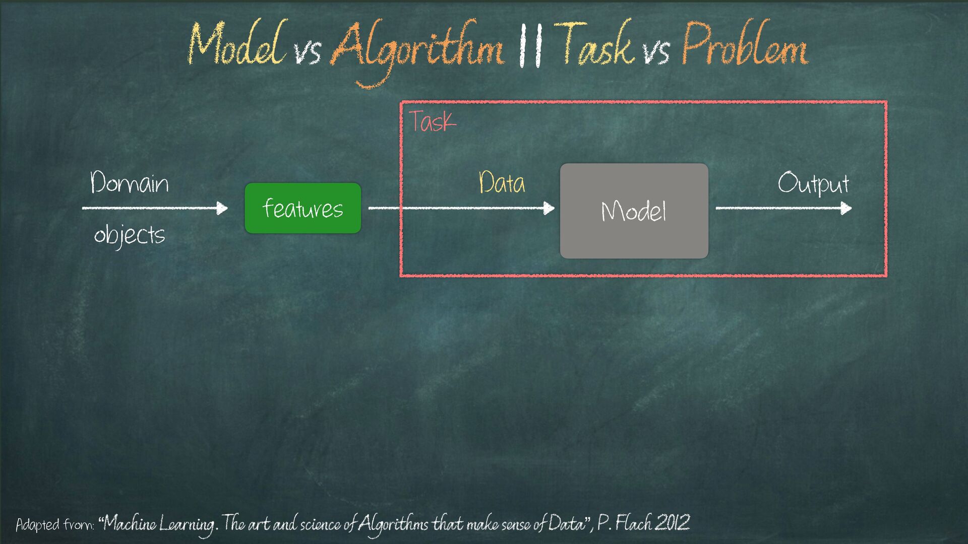
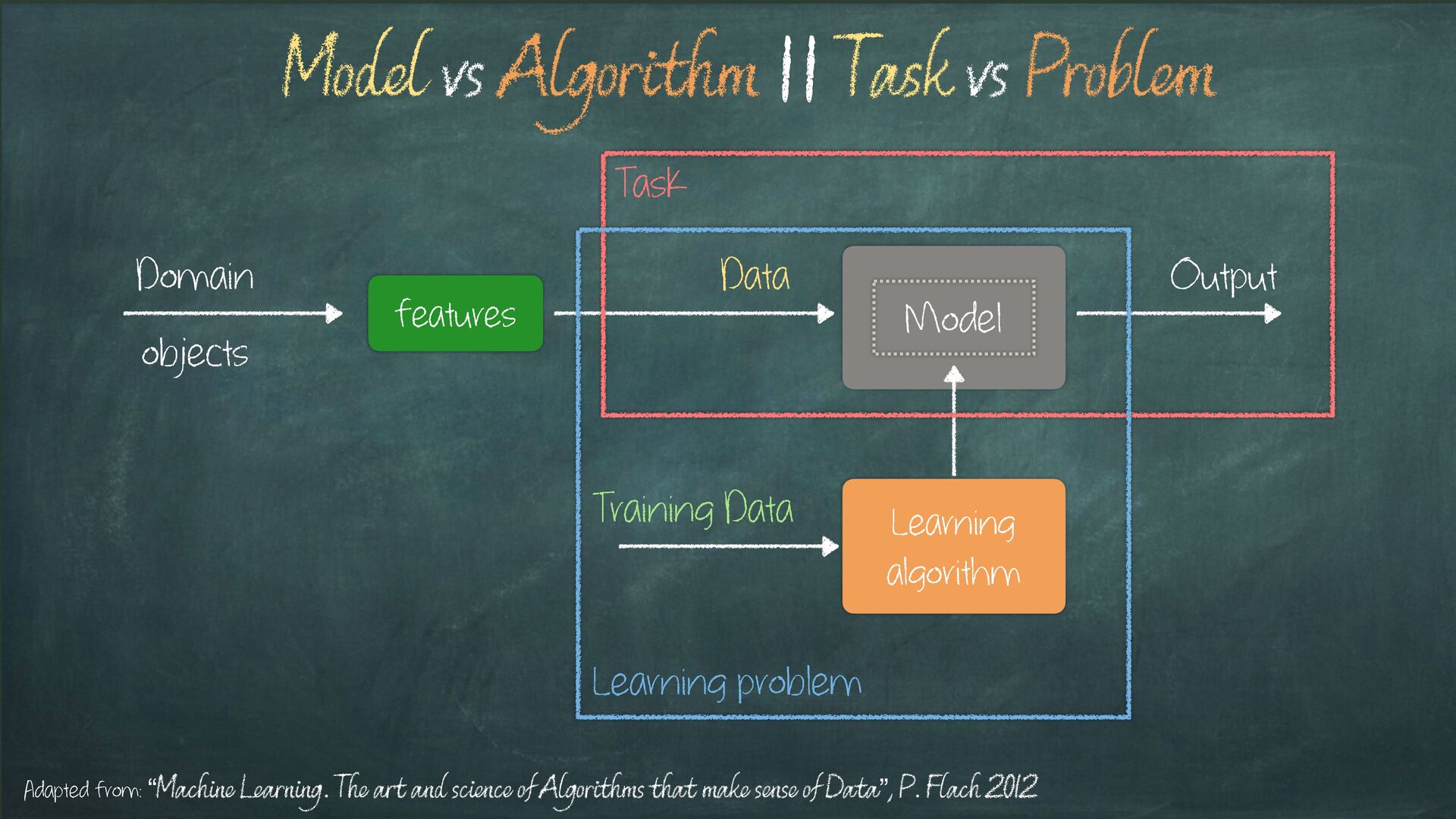
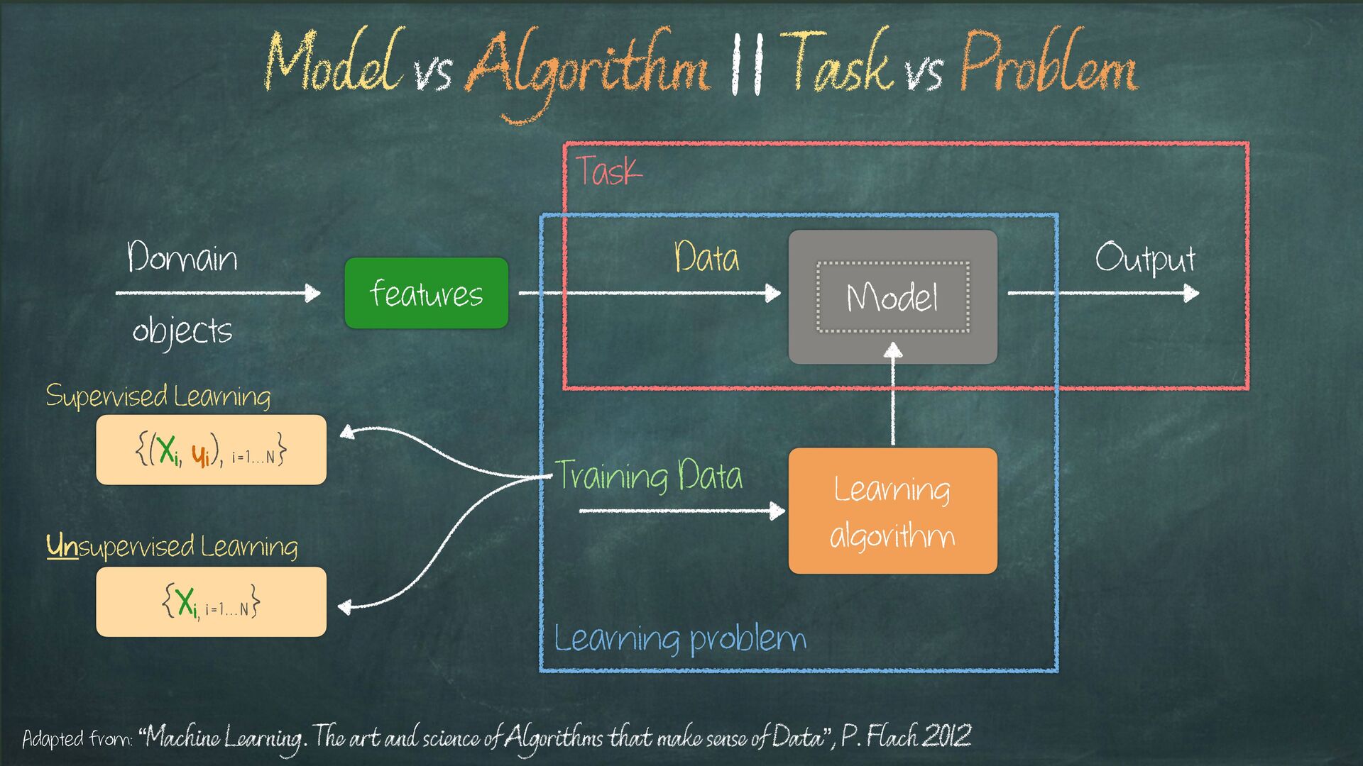
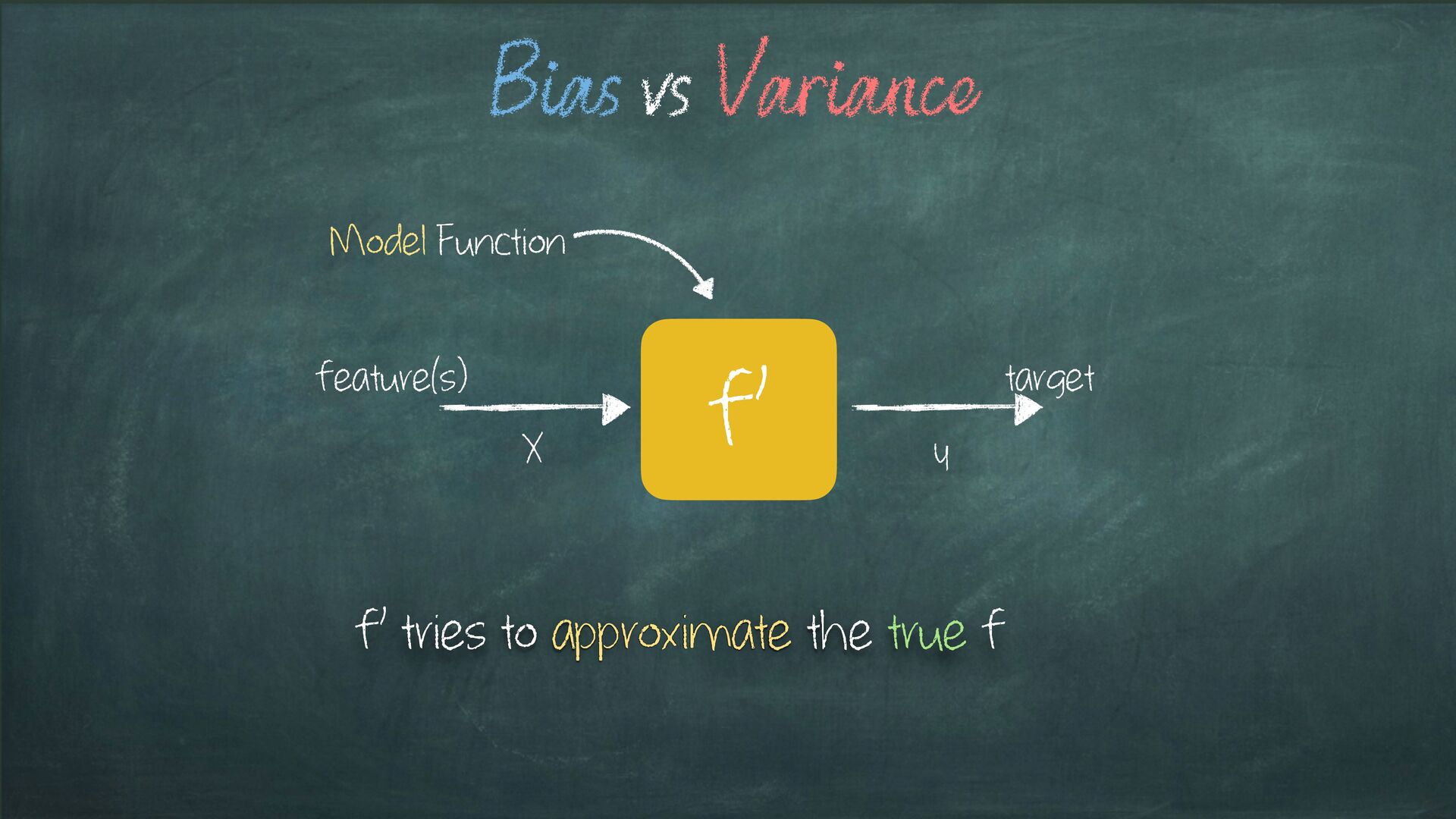
Learning problem Task Model vs Algorithm || Task vs Problem Adapted from: “Machine Learning. The art and science of Algorithms that make sense of Data”, P. Flach 2012
Learning problem Task Model vs Algorithm || Task vs Problem Adapted from: “Machine Learning. The art and science of Algorithms that make sense of Data”, P. Flach 2012 {(Xi, yi), i = 1 , . . N } {Xi, i = 1 , . . N } Supervised Learning Unsupervised Learning
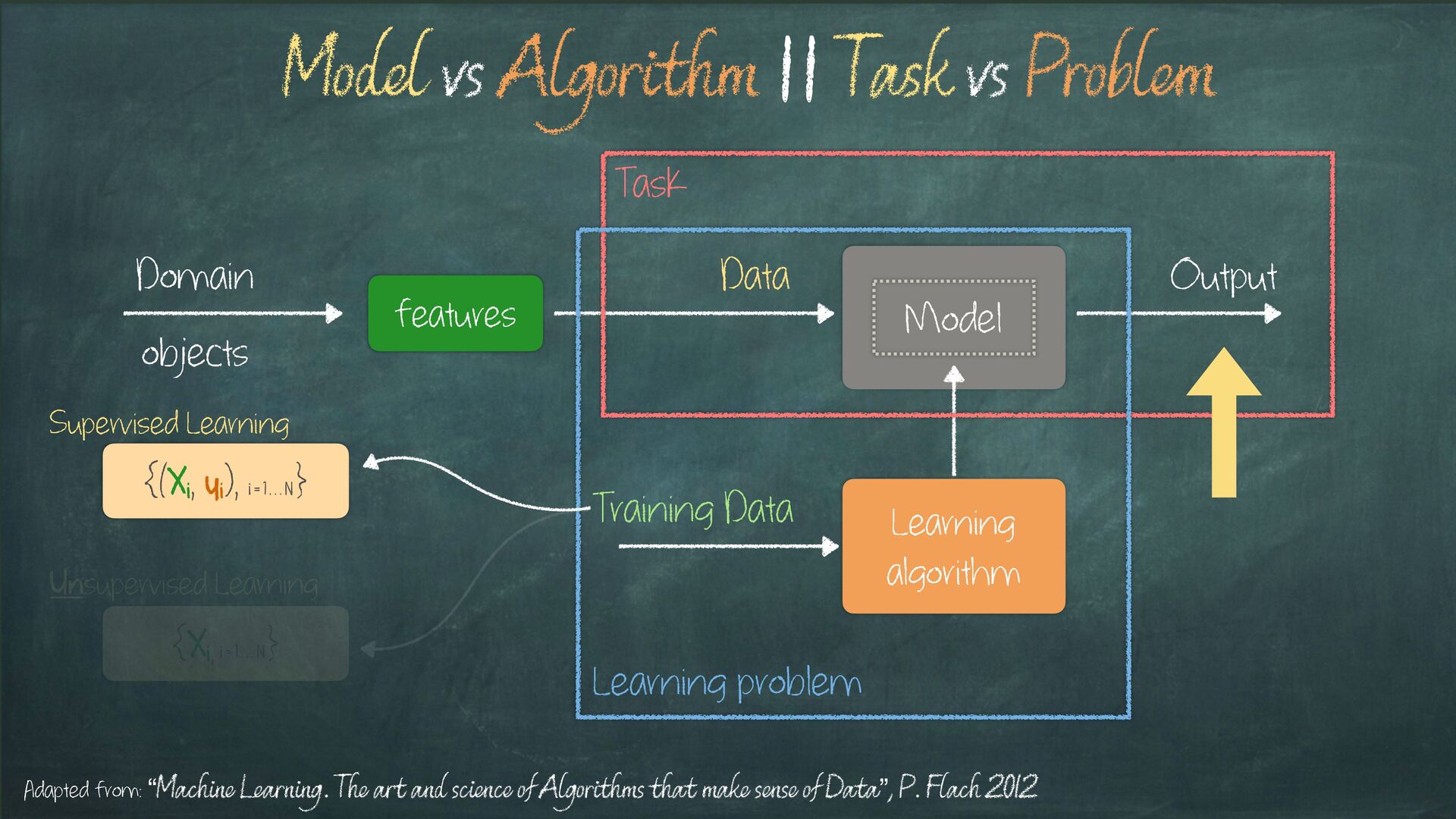
Learning problem Task Model vs Algorithm || Task vs Problem Adapted from: “Machine Learning. The art and science of Algorithms that make sense of Data”, P. Flach 2012 {(Xi, yi), i = 1 , . . N } {Xi, i = 1 , . . N } Supervised Learning Unsupervised Learning
are required to carry out a Machine Learning Experiment (see next slide) Basic components !" Recipes Aim #2: Give you some appreciation of the importance of choosing measurements that are appropriate for your particular experiment e.g. (just) Accuracy may not be the right metric to use! Learning Objectives
(D) Common Examples of RQs are: How does model m perform on data from domain D Much harder: How m would (also) perform on data from D2 (!" D) Which of these models m1, m2, … mk from A has the best performance on data from D Which of these learning algorithms gives the best model on data from D Machine Learning Experiment
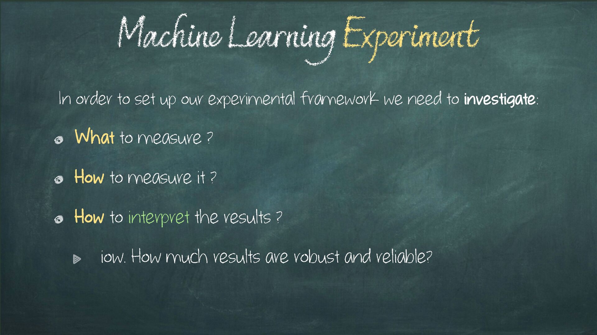
to interpret the results ? iow. How much results are robust and reliable? Machine Learning Experiment In order to set up our experimental framework we need to investigate:
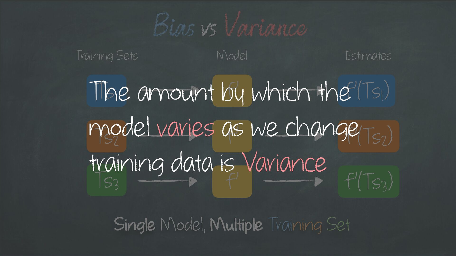
vs Variance Single Model, Multiple Training Set Model Training Sets Estimates The amount by which the model varies as we change training data is Variance
to interpret the results ? iow. How much results are robust and reliable? Machine Learning Experiment In order to set up our experimental framework we need to investigate:
a Binary Classification Problem (we’re still in the Supervised learning territory) True Positive TP True Negative TN False Negative FN False Positive FP True Class Predicated Class Positive Negative Positive Negative Confusion Matrix (In clockwise order…)
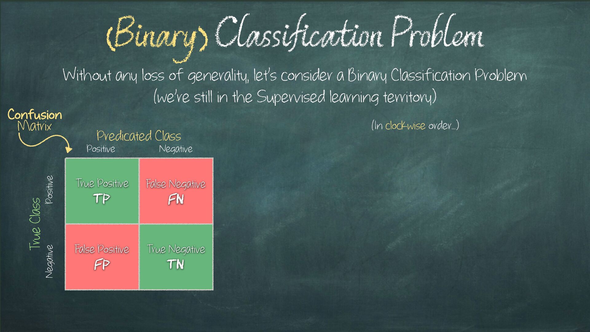
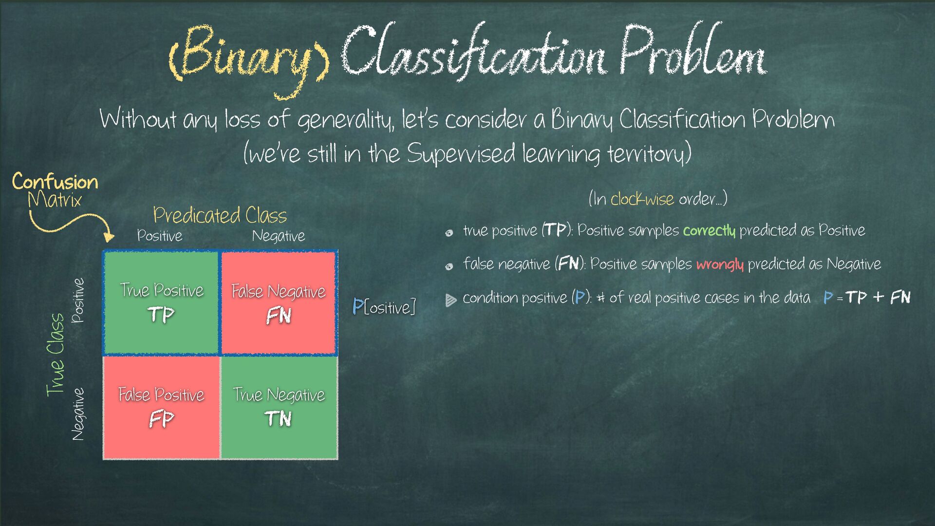
Classification Problem Without any loss of generality, let’s consider a Binary Classification Problem (we’re still in the Supervised learning territory) True Positive TP True Negative TN False Negative FN False Positive FP True Class Predicated Class Positive Negative Positive Negative Confusion Matrix (In clockwise order…)
negative (FN): Positive samples wrongly predicted as Negative (Binary) Classification Problem Without any loss of generality, let’s consider a Binary Classification Problem (we’re still in the Supervised learning territory) True Positive TP True Negative TN False Negative FN False Positive FP True Class Predicated Class Positive Negative Positive Negative Confusion Matrix (In clockwise order…)
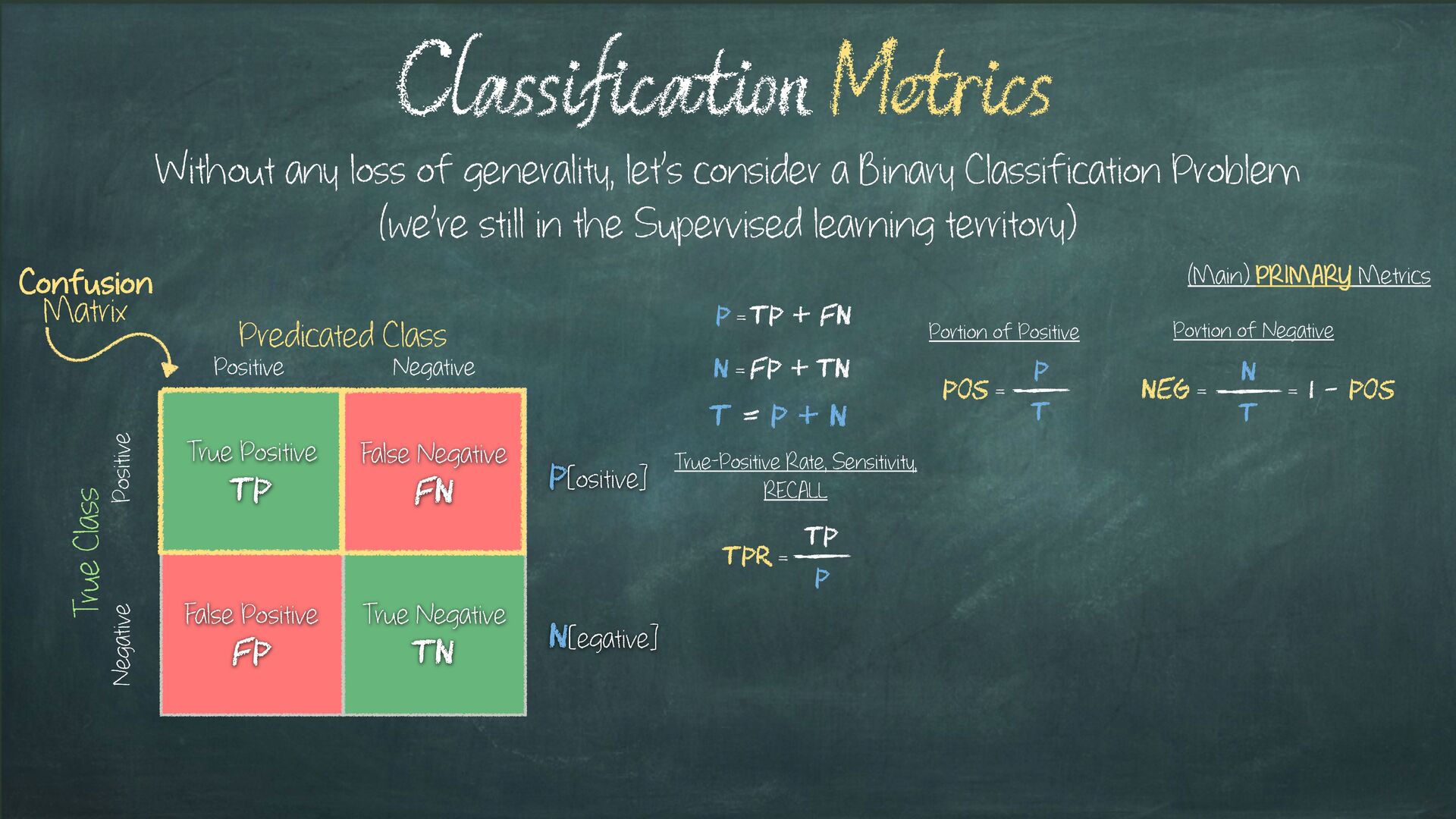
negative (FN): Positive samples wrongly predicted as Negative condition positive (P): # of real positive cases in the data (Binary) Classification Problem Without any loss of generality, let’s consider a Binary Classification Problem (we’re still in the Supervised learning territory) True Positive TP True Negative TN False Negative FN False Positive FP True Class Predicated Class Positive Negative Positive Negative Confusion Matrix P[ositive] P = TP + FN (In clockwise order…)
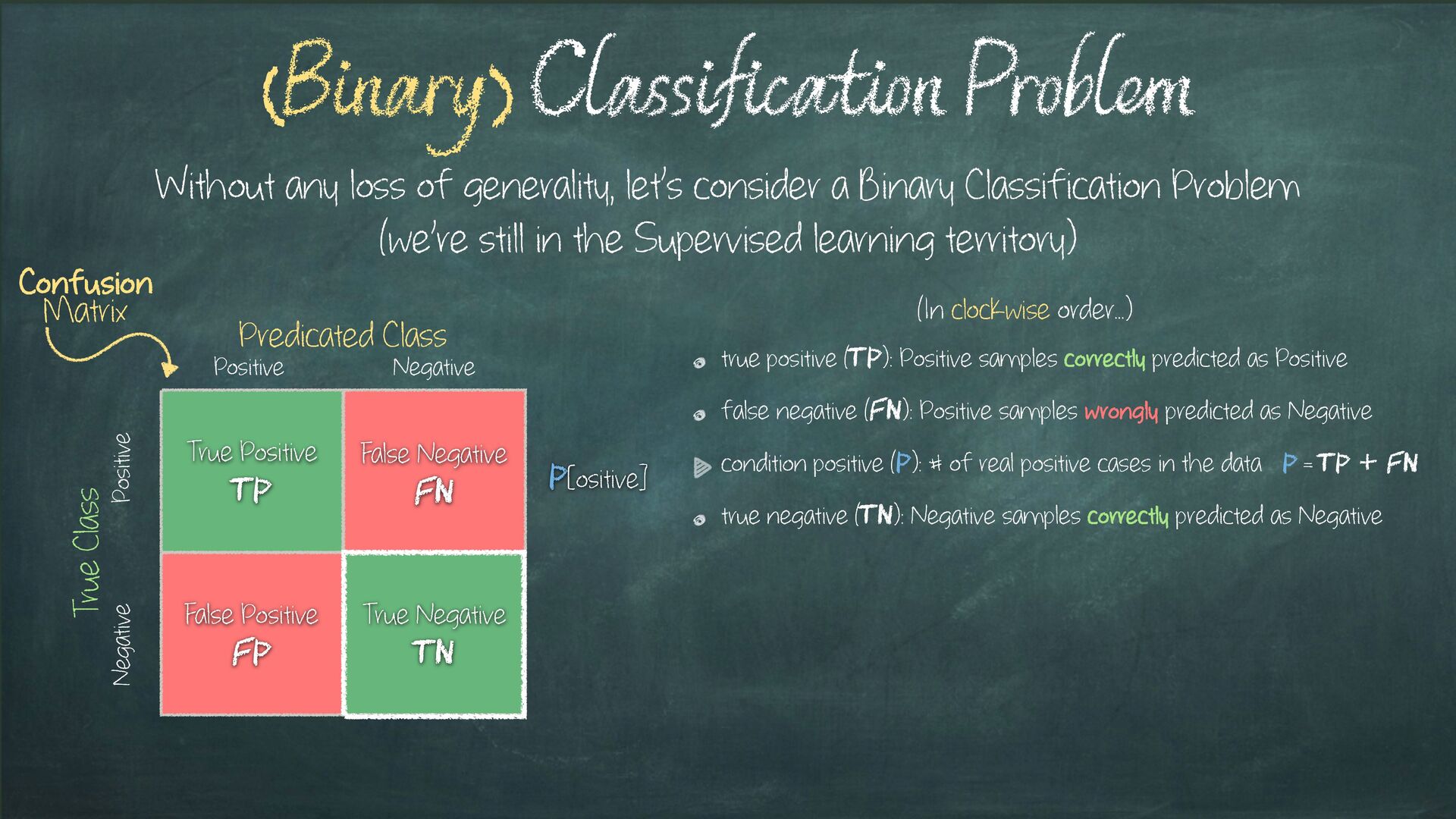
negative (FN): Positive samples wrongly predicted as Negative condition positive (P): # of real positive cases in the data true negative (TN): Negative samples correctly predicted as Negative (Binary) Classification Problem Without any loss of generality, let’s consider a Binary Classification Problem (we’re still in the Supervised learning territory) True Positive TP True Negative TN False Negative FN False Positive FP True Class Predicated Class Positive Negative Positive Negative Confusion Matrix P[ositive] P = TP + FN (In clockwise order…)
negative (FN): Positive samples wrongly predicted as Negative condition positive (P): # of real positive cases in the data true negative (TN): Negative samples correctly predicted as Negative false positive (FP): Negative samples wrongly predicted as Positive (Binary) Classification Problem Without any loss of generality, let’s consider a Binary Classification Problem (we’re still in the Supervised learning territory) True Positive TP True Negative TN False Negative FN False Positive FP True Class Predicated Class Positive Negative Positive Negative Confusion Matrix P[ositive] P = TP + FN (In clockwise order…)
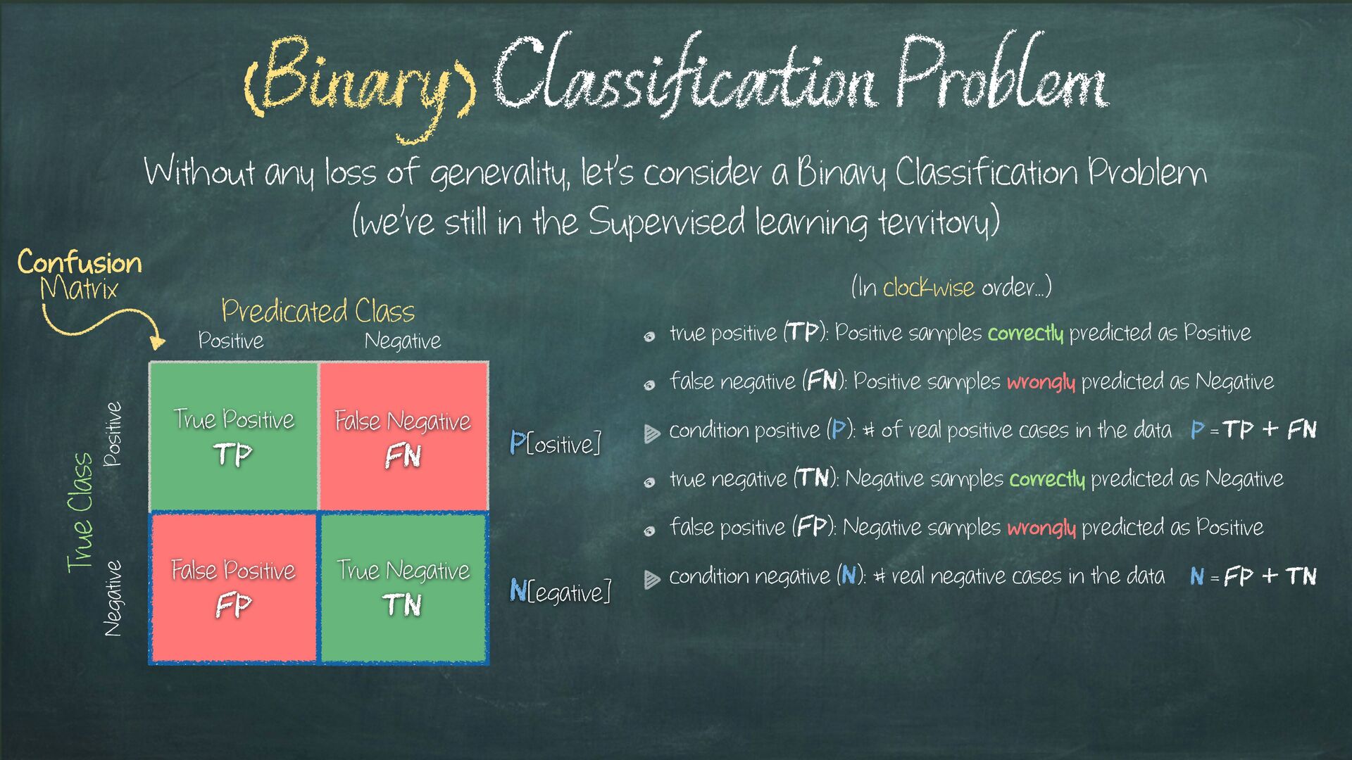
negative (FN): Positive samples wrongly predicted as Negative condition positive (P): # of real positive cases in the data true negative (TN): Negative samples correctly predicted as Negative false positive (FP): Negative samples wrongly predicted as Positive condition negative (N): # real negative cases in the data (Binary) Classification Problem Without any loss of generality, let’s consider a Binary Classification Problem (we’re still in the Supervised learning territory) True Positive TP True Negative TN False Negative FN False Positive FP True Class Predicated Class Positive Negative Positive Negative Confusion Matrix P[ositive] N[egative] N = FP + TN P = TP + FN (In clockwise order…)
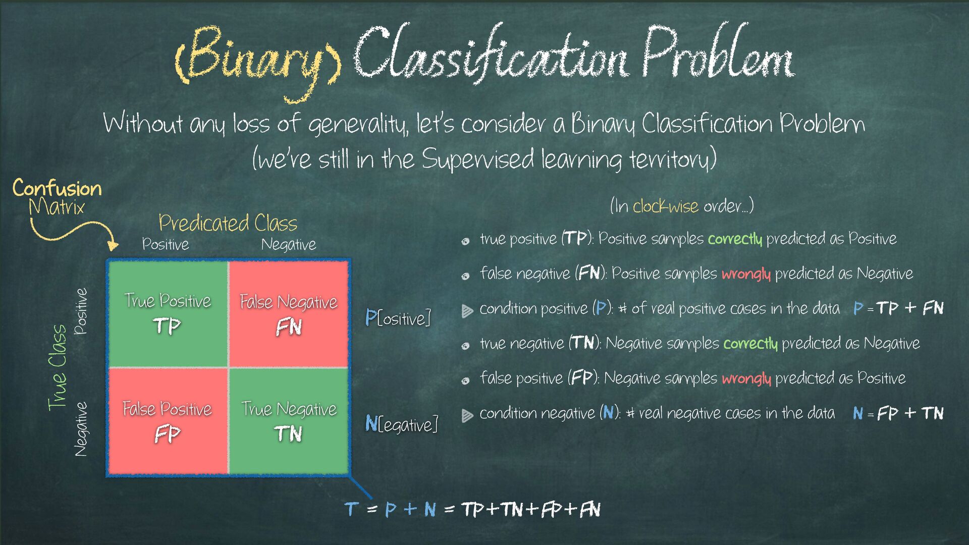
negative (FN): Positive samples wrongly predicted as Negative condition positive (P): # of real positive cases in the data true negative (TN): Negative samples correctly predicted as Negative false positive (FP): Negative samples wrongly predicted as Positive condition negative (N): # real negative cases in the data (Binary) Classification Problem Without any loss of generality, let’s consider a Binary Classification Problem (we’re still in the Supervised learning territory) True Positive TP True Negative TN False Negative FN False Positive FP True Class Predicated Class Positive Negative Positive Negative Confusion Matrix P[ositive] N[egative] N = FP + TN P = TP + FN T = P + N = TP + TN + FP + FN (In clockwise order…)
negative (FN): Positive samples wrongly predicted as Negative condition positive (P): # of real positive cases in the data true negative (TN): Negative samples correctly predicted as Negative false positive (FP): Negative samples wrongly predicted as Positive condition negative (N): # real negative cases in the data (Binary) Classification Problem Without any loss of generality, let’s consider a Binary Classification Problem (we’re still in the Supervised learning territory) True Positive TP True Negative TN False Negative FN False Positive FP True Class Predicated Class Positive Negative Positive Negative Confusion Matrix P[ositive] N[egative] N = FP + TN P = TP + FN T = P + N = TP + TN + FP + FN (In clockwise order…) Portion of Positive Pos = P T
negative (FN): Positive samples wrongly predicted as Negative condition positive (P): # of real positive cases in the data true negative (TN): Negative samples correctly predicted as Negative false positive (FP): Negative samples wrongly predicted as Positive condition negative (N): # real negative cases in the data (Binary) Classification Problem Without any loss of generality, let’s consider a Binary Classification Problem (we’re still in the Supervised learning territory) True Positive TP True Negative TN False Negative FN False Positive FP True Class Predicated Class Positive Negative Positive Negative Confusion Matrix P[ositive] N[egative] N = FP + TN P = TP + FN T = P + N = TP + TN + FP + FN (In clockwise order…) Portion of Positive Pos = P T Portion of Negative Neg = = 1 - POS N T
Positive FP True Class Predicated Class Positive Negative Positive Negative Confusion Matrix Classification Metrics Without any loss of generality, let’s consider a Binary Classification Problem (we’re still in the Supervised learning territory) P[ositive] N[egative] N = FP + TN P = TP + FN T = P + N Portion of Positive Pos = P T Portion of Negative Neg = = 1 - POS N T (Main) PRIMARY Metrics
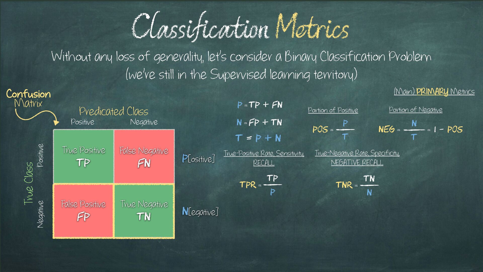
Positive FP True Class Predicated Class Positive Negative Positive Negative Confusion Matrix Classification Metrics Without any loss of generality, let’s consider a Binary Classification Problem (we’re still in the Supervised learning territory) TPR = TP P True-Positive Rate, Sensitivity, RECALL P[ositive] N[egative] N = FP + TN P = TP + FN T = P + N Portion of Positive Pos = P T Portion of Negative Neg = = 1 - POS N T (Main) PRIMARY Metrics
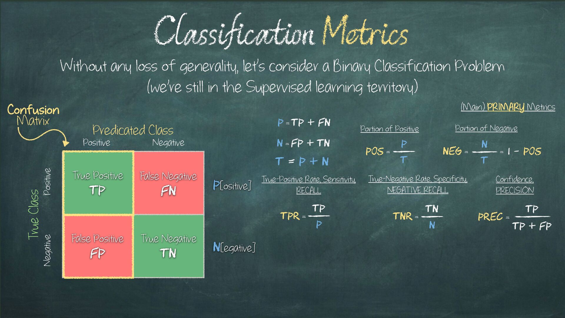
Positive FP True Class Predicated Class Positive Negative Positive Negative Confusion Matrix Classification Metrics Without any loss of generality, let’s consider a Binary Classification Problem (we’re still in the Supervised learning territory) TPR = TP P True-Positive Rate, Sensitivity, RECALL True-Negative Rate, Specificity, NEGATIVE RECALL TNR = TN N P[ositive] N[egative] N = FP + TN P = TP + FN T = P + N Portion of Positive Pos = P T Portion of Negative Neg = = 1 - POS N T (Main) PRIMARY Metrics
Positive FP True Class Predicated Class Positive Negative Positive Negative Confusion Matrix Classification Metrics Without any loss of generality, let’s consider a Binary Classification Problem (we’re still in the Supervised learning territory) TPR = TP P True-Positive Rate, Sensitivity, RECALL True-Negative Rate, Specificity, NEGATIVE RECALL TNR = TN N Confidence, PRECISION PREC = TP TP + FP P[ositive] N[egative] N = FP + TN P = TP + FN T = P + N Portion of Positive Pos = P T Portion of Negative Neg = = 1 - POS N T (Main) PRIMARY Metrics
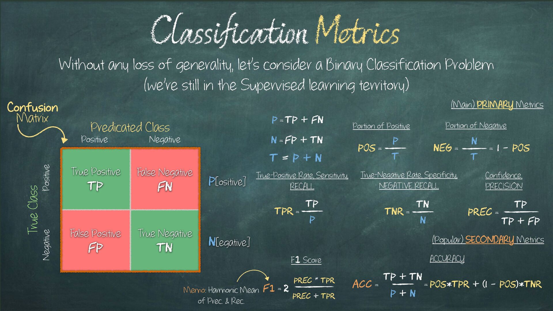
Positive FP True Class Predicated Class Positive Negative Positive Negative Confusion Matrix Classification Metrics Without any loss of generality, let’s consider a Binary Classification Problem (we’re still in the Supervised learning territory) TPR = TP P True-Positive Rate, Sensitivity, RECALL True-Negative Rate, Specificity, NEGATIVE RECALL TNR = TN N Confidence, PRECISION PREC = TP TP + FP F1 Score F1 = 2 PREC + TPR PREC * TPR Memo: Harmonic Mean of Prec. & Rec. P[ositive] N[egative] N = FP + TN P = TP + FN T = P + N Portion of Positive Pos = P T Portion of Negative Neg = = 1 - POS N T (Popular) SECONDARY Metrics (Main) PRIMARY Metrics
Positive FP True Class Predicated Class Positive Negative Positive Negative Confusion Matrix Classification Metrics Without any loss of generality, let’s consider a Binary Classification Problem (we’re still in the Supervised learning territory) TPR = TP P True-Positive Rate, Sensitivity, RECALL True-Negative Rate, Specificity, NEGATIVE RECALL TNR = TN N Confidence, PRECISION PREC = TP TP + FP F1 Score F1 = 2 PREC + TPR PREC * TPR Memo: Harmonic Mean of Prec. & Rec. P[ositive] N[egative] N = FP + TN P = TP + FN T = P + N Portion of Positive Pos = P T Portion of Negative Neg = = 1 - POS N T ACC = TP + TN P + N = POS*TPR + (1 - POS)*TNR ACCURACY (Popular) SECONDARY Metrics (Main) PRIMARY Metrics
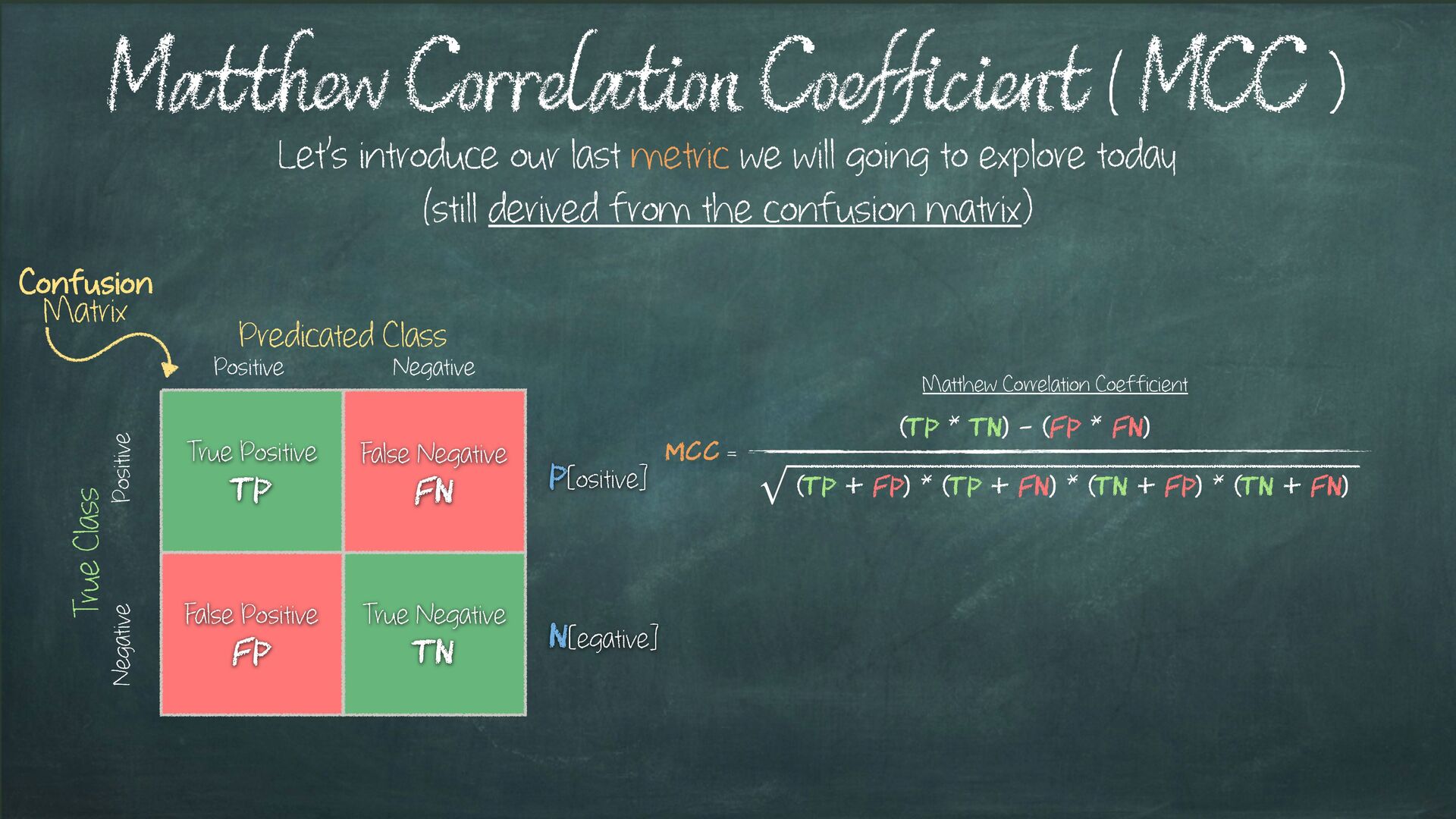
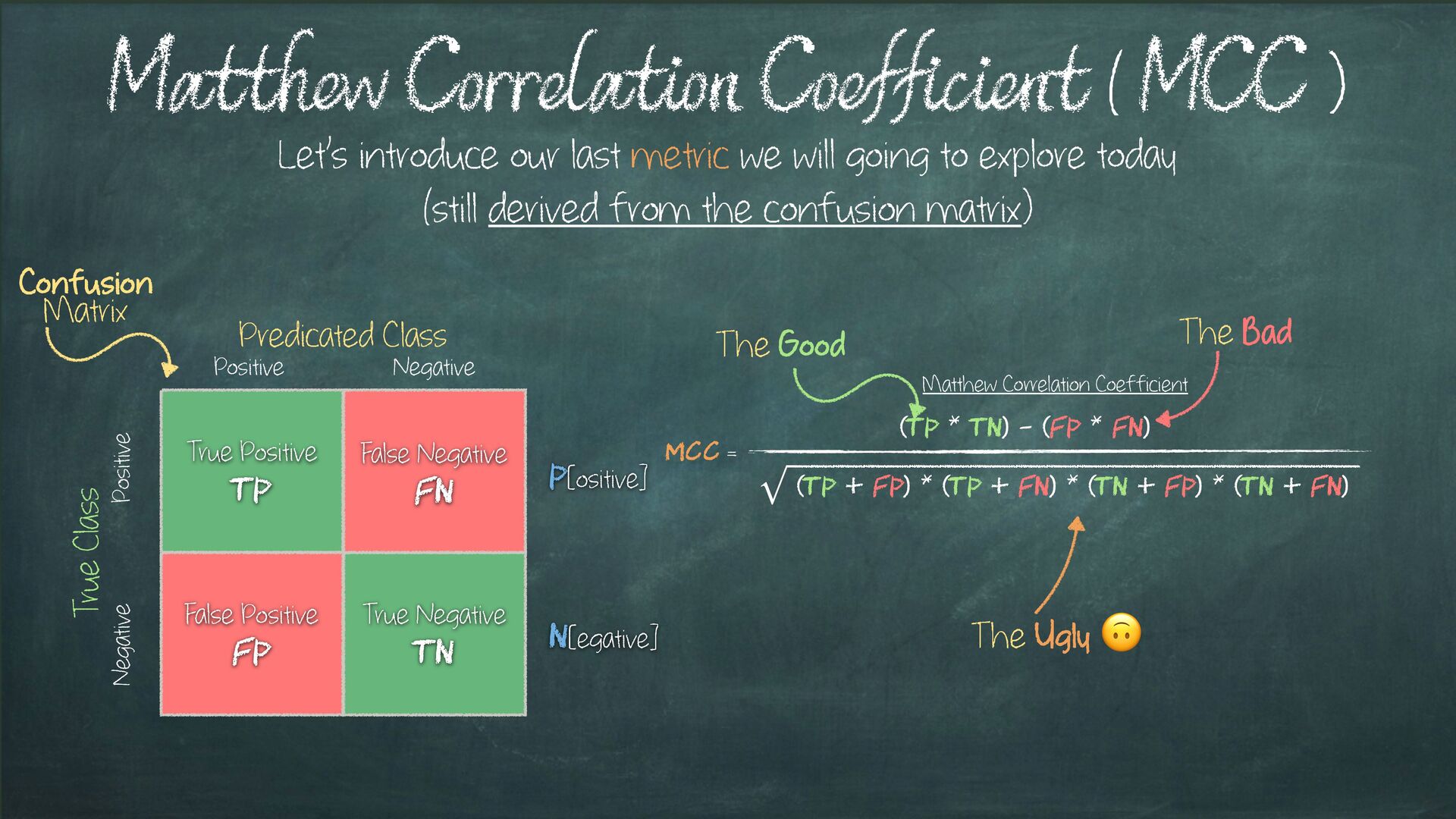
Positive FP True Class Predicated Class Positive Negative Positive Negative Confusion Matrix Matthew Correlation Coefficient ( MCC ) Let’s introduce our last metric we will going to explore today (still derived from the confusion matrix) P[ositive] N[egative] MCC = (TP * TN) - (FP * FN) Matthew Correlation Coefficient (TP + FP) * (TP + FN) * (TN + FP) * (TN + FN) The Good The Bad The Ugly !
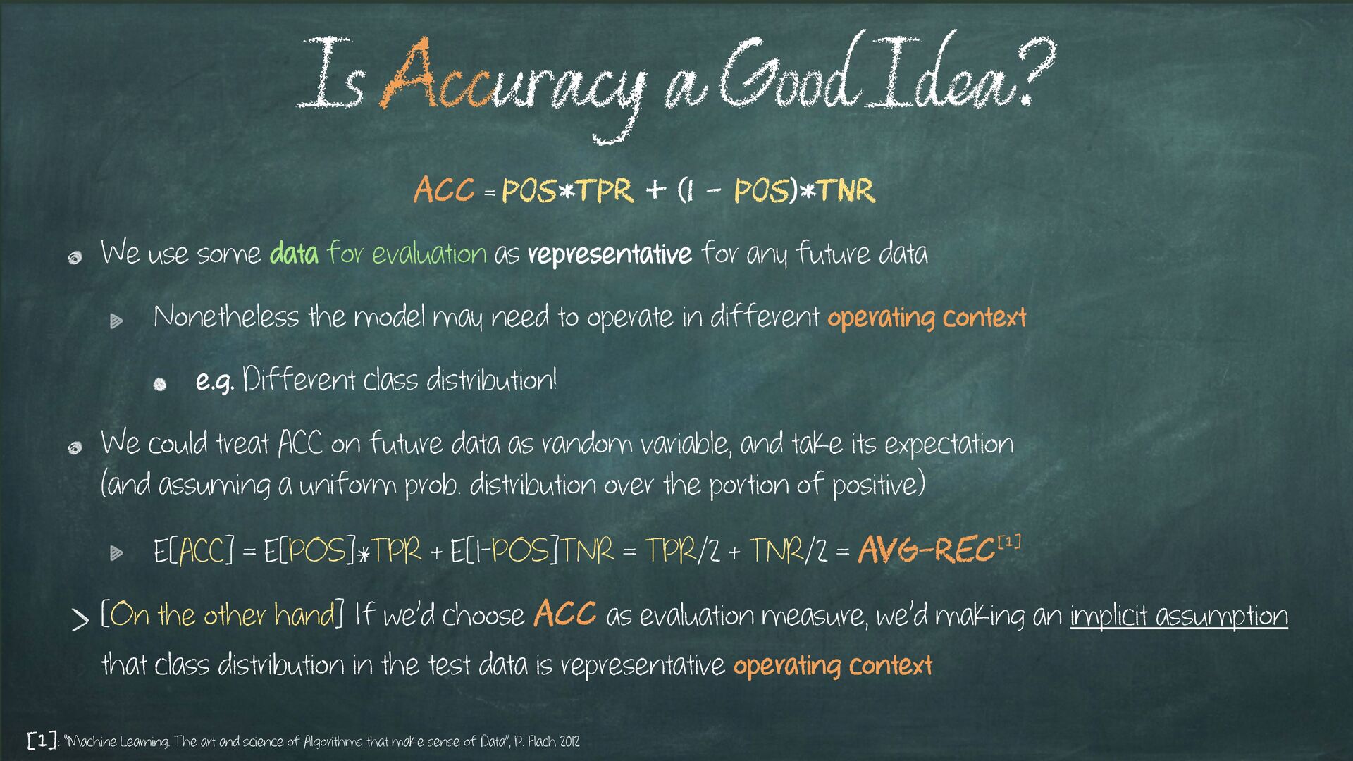
future data Nonetheless the model may need to operate in different operating context e.g. Different class distribution! We could treat ACC on future data as random variable, and take its expectation (and assuming a uniform prob. distribution over the portion of positive) E[ACC] = E[POS]*TPR + E[1-POS]TNR = TPR/2 + TNR/2 = AVG-REC[1] [On the other hand] If we’d choose ACC as evaluation measure, we’d making an implicit assumption that class distribution in the test data is representative operating context Is Accuracy a Good Idea? ACC = POS*TPR + (1 - POS)*TNR [1]: “Machine Learning. The art and science of Algorithms that make sense of Data”, P. Flach 2012
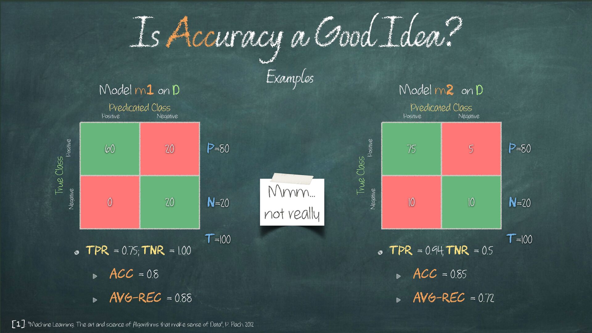
= 0.88 Is Accuracy a Good Idea? 60 20 20 0 True Class Predicated Class Positive Negative Positive Negative T=100 P=80 N=20 Examples Model m1 on D 75 10 5 10 True Class Predicated Class Positive Negative Positive Negative T=100 P=80 N=20 Model m2 on D TPR = 0.94; TNR = 0.5 ACC = 0.85 AVG-REC = 0.72 [1]: “Machine Learning. The art and science of Algorithms that make sense of Data”, P. Flach 2012 Mmm… not really
art and science of Algorithms that make sense of Data”, P. Flach 2012 TPR = TP P RECALL PRECISION PREC = TP TP + FP F1 Score (Harmonic Mean) F1 = 2 PREC + TPR PREC * TPR 75 10 5 10 True Class Predicated Class Positive Negative Positive Negative T=100 P=80 N=20 Model m2 on D PREC = 75 / 85 = 0.88; TPR = 75 / 80 = 0.94 F1 = 0.91 ACC = 0.85 75 910 5 10 True Class Predicated Class Positive Negative Positive Negative T=1000 P=80 N=920 Model m2 on D2 PREC = 75 / 85 = 0.88; TPR = 75 / 80 = 0.94 F1 = 0.91 ACC = 0.99 F1 to be preferred in domains where negatives abound (and are not the relevant class)
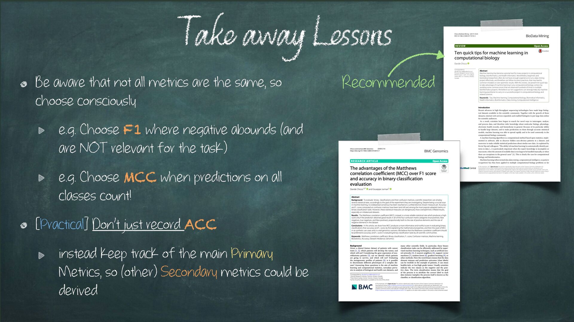
choose consciously e.g. Choose F1 where negative abounds (and are NOT relevant for the task) e.g. Choose MCC when predictions on all classes count! [Practical] Don’t just record ACC instead keep track of the main Primary Metrics, so (other) Secondary metrics could be derived Take away Lessons Recommended
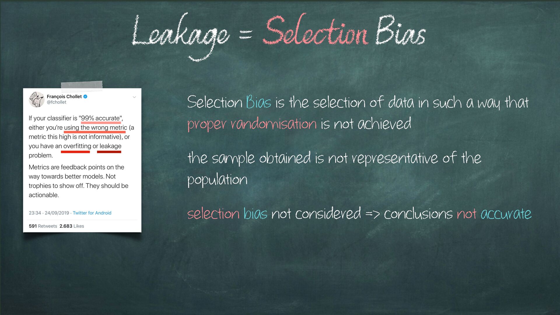
way that proper randomisation is not achieved the sample obtained is not representative of the population selection bias not considered => conclusions not accurate Leakage = Selection Bias
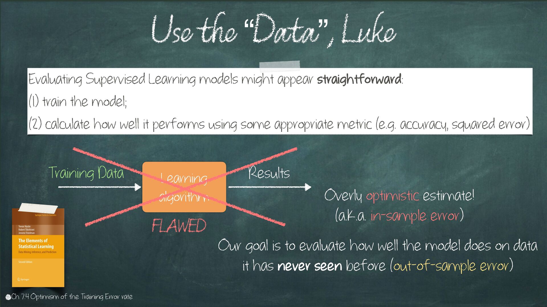
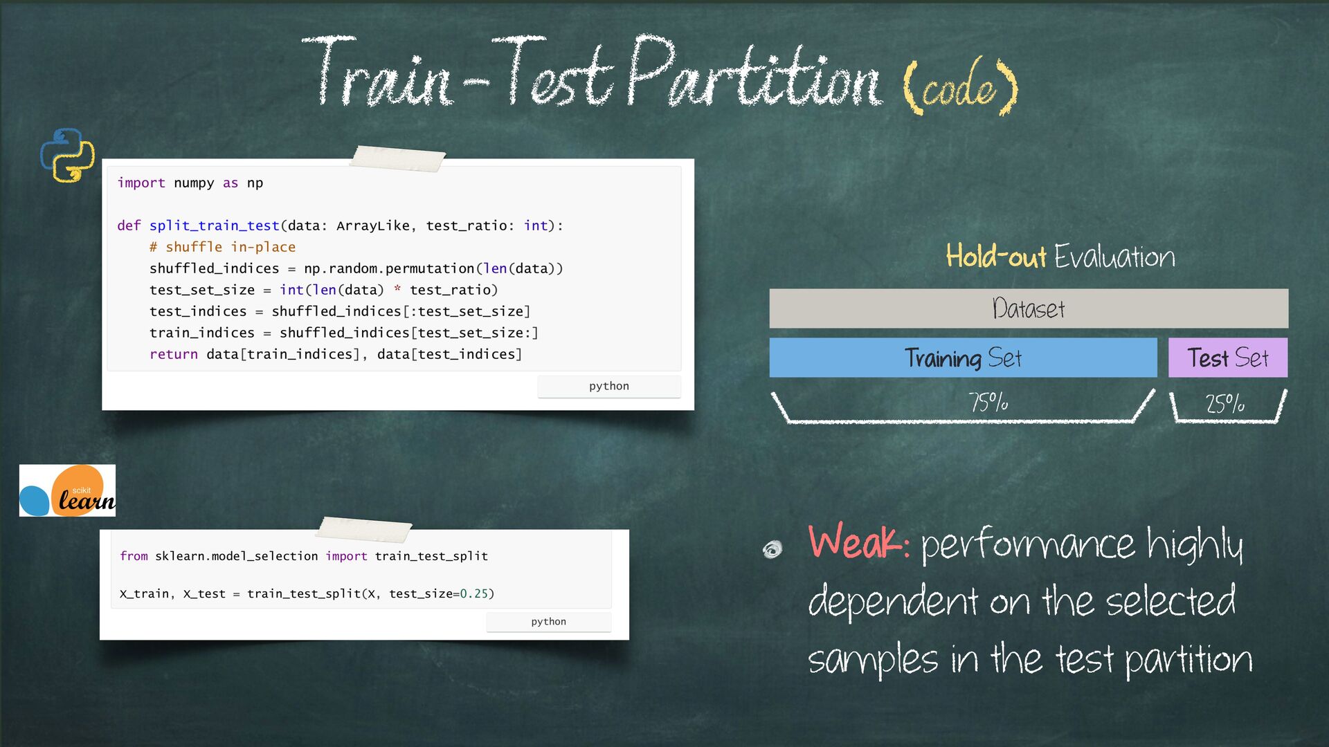
straightforward: (1) train the model; (2) calculate how well it performs using some appropriate metric (e.g. accuracy, squared error) Learning algorithm Training Data Results FLAWED Our goal is to evaluate how well the model does on data it has never seen before (out-of-sample error) Overly optimistic estimate! (a.k.a. in-sample error) Ch 7.4 Optimism of the Training Error rate
this (time series) data (A) poor Training Subset (B) good Training Subset Examples (1) (A) also invalidates the i.i.d. assumption! Independent and Identically distributed
poor Validation Subset A good Validation Subset Whole Slide Images Detect Tissue Region Subject split Train Test Random split Train Test Tiles Train-Test Split [1]: “AI slipping on tiles: data leakage in digital pathology”, Bussola, Marcolini, Maggio, et al. - https://arxiv.org/abs/1909.06539 Sampling Bias (or selection Bias) Examples (2)
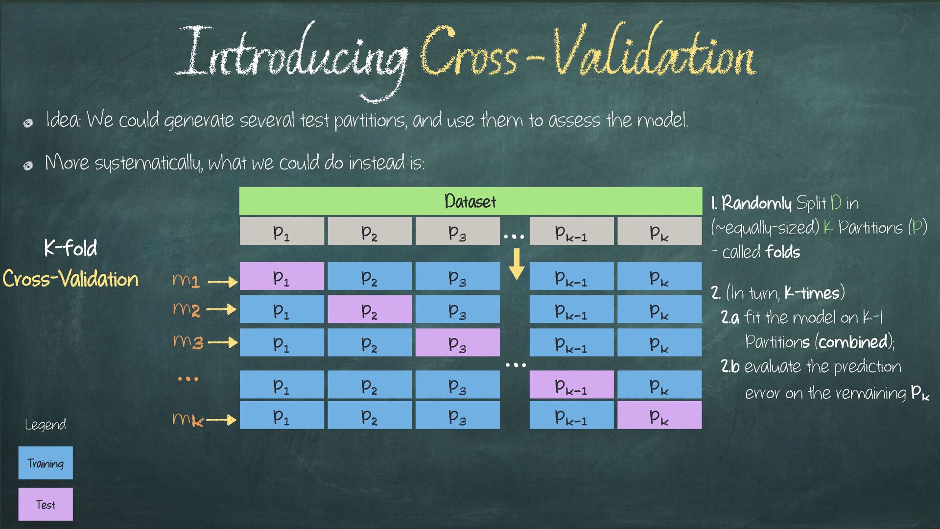
to assess the model. More systematically, what we could do instead is: Introducing Cross-Validation K-fold Cross-Validation Dataset Pk P1 P2 P3 Pk-1 … Pk P1 P2 P3 Pk-1 Pk P1 P2 P3 Pk-1 Pk P1 P2 P3 Pk-1 Pk P1 P2 P3 Pk-1 Pk P1 P2 P3 Pk-1 … Test Training Legend 1. Randomly Split D in (~equally-sized) k Partitions (P) - called folds 2. (In turn, k-times) 2.a fit the model on k-1 Partitions (combined); 2.b evaluate the prediction error on the remaining Pk m1 m2 m3 … mk
to assess the model. More systematically, what we could do instead is: Introducing Cross-Validation K-fold Cross-Validation Dataset Pk P1 P2 P3 Pk-1 … Pk P1 P2 P3 Pk-1 Pk P1 P2 P3 Pk-1 Pk P1 P2 P3 Pk-1 Pk P1 P2 P3 Pk-1 Pk P1 P2 P3 Pk-1 … Test Training Legend 1. Randomly Split D in (~equally-sized) k Partitions (P) - called folds 2. (In turn, k-times) 2.a fit the model on k-1 Partitions (combined); 2.b evaluate the prediction error on the remaining Pk m1 m2 m3 … mk CV(A,D) = 1 K Σ K i=1 Åi = metric( mi, Pi )
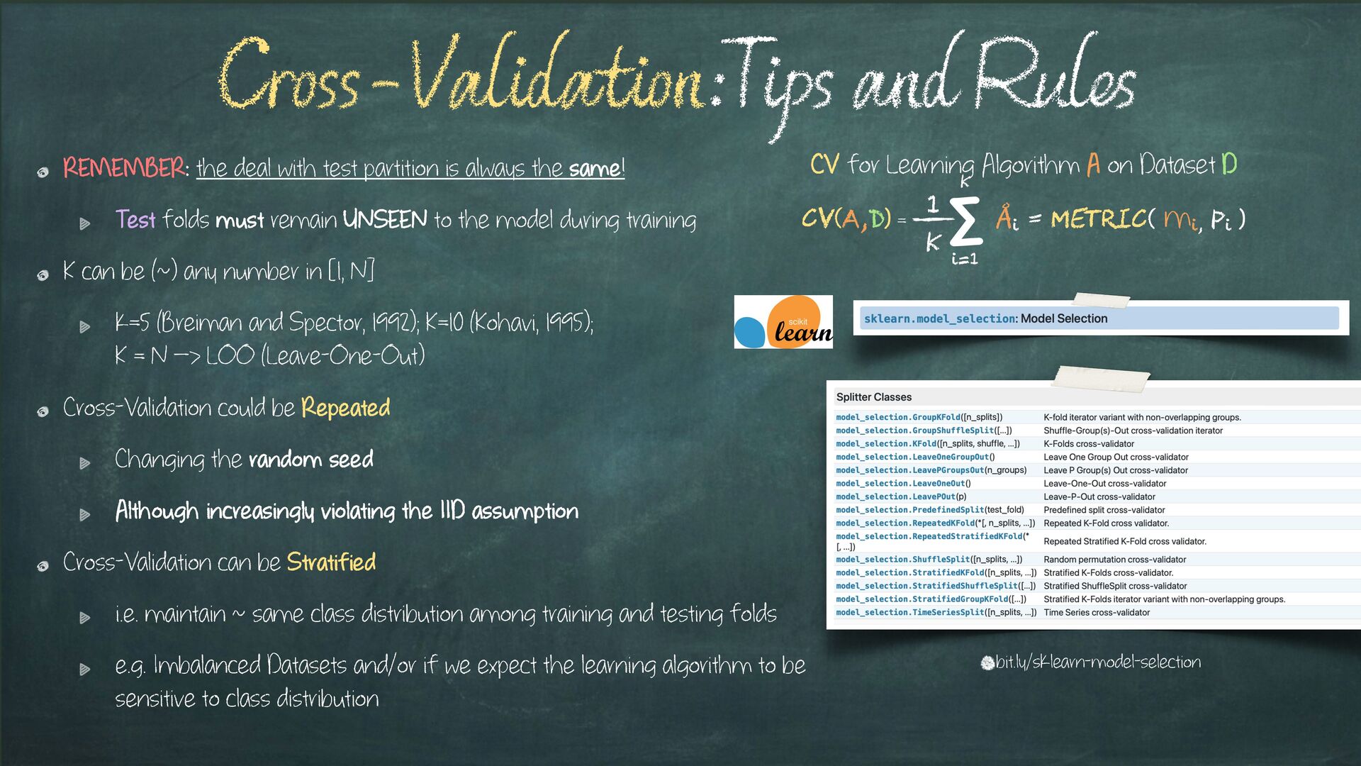
Test folds must remain UNSEEN to the model during training K can be (~) any number in [1, N] k=5 (Breiman and Spector, 1992); K=10 (Kohavi, 1995); K = N —> LOO (Leave-One-Out) Cross-Validation could be Repeated Changing the random seed Although increasingly violating the IID assumption Cross-Validation can be Stratified i.e. maintain ~ same class distribution among training and testing folds e.g. Imbalanced Datasets and/or if we expect the learning algorithm to be sensitive to class distribution Cross-Validation:Tips and Rules bit.ly/sklearn-model-selection CV for Learning Algorithm A on Dataset D CV(A,D) = 1 K Σ K i=1 Åi = metric( mi, Pi )
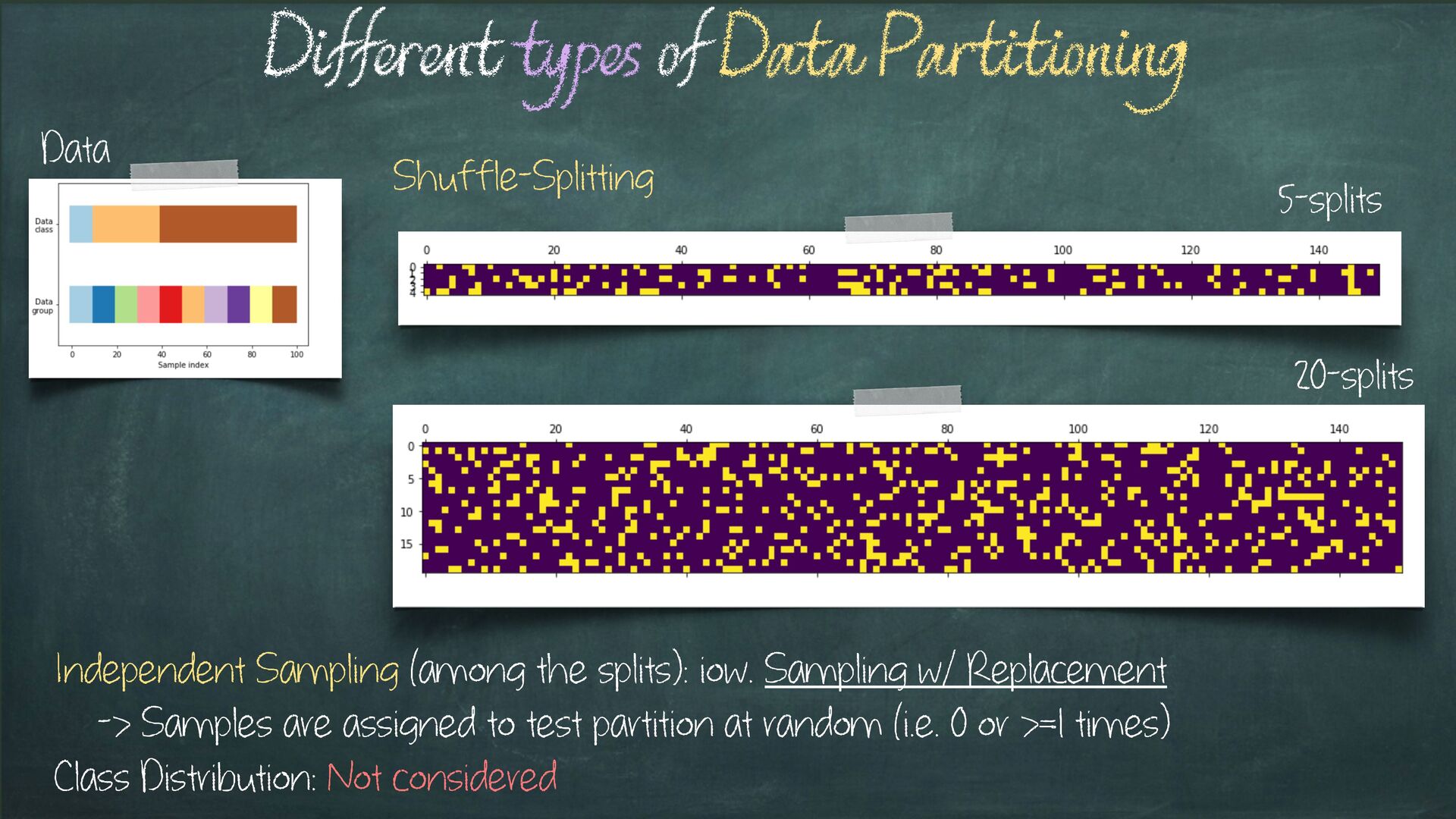
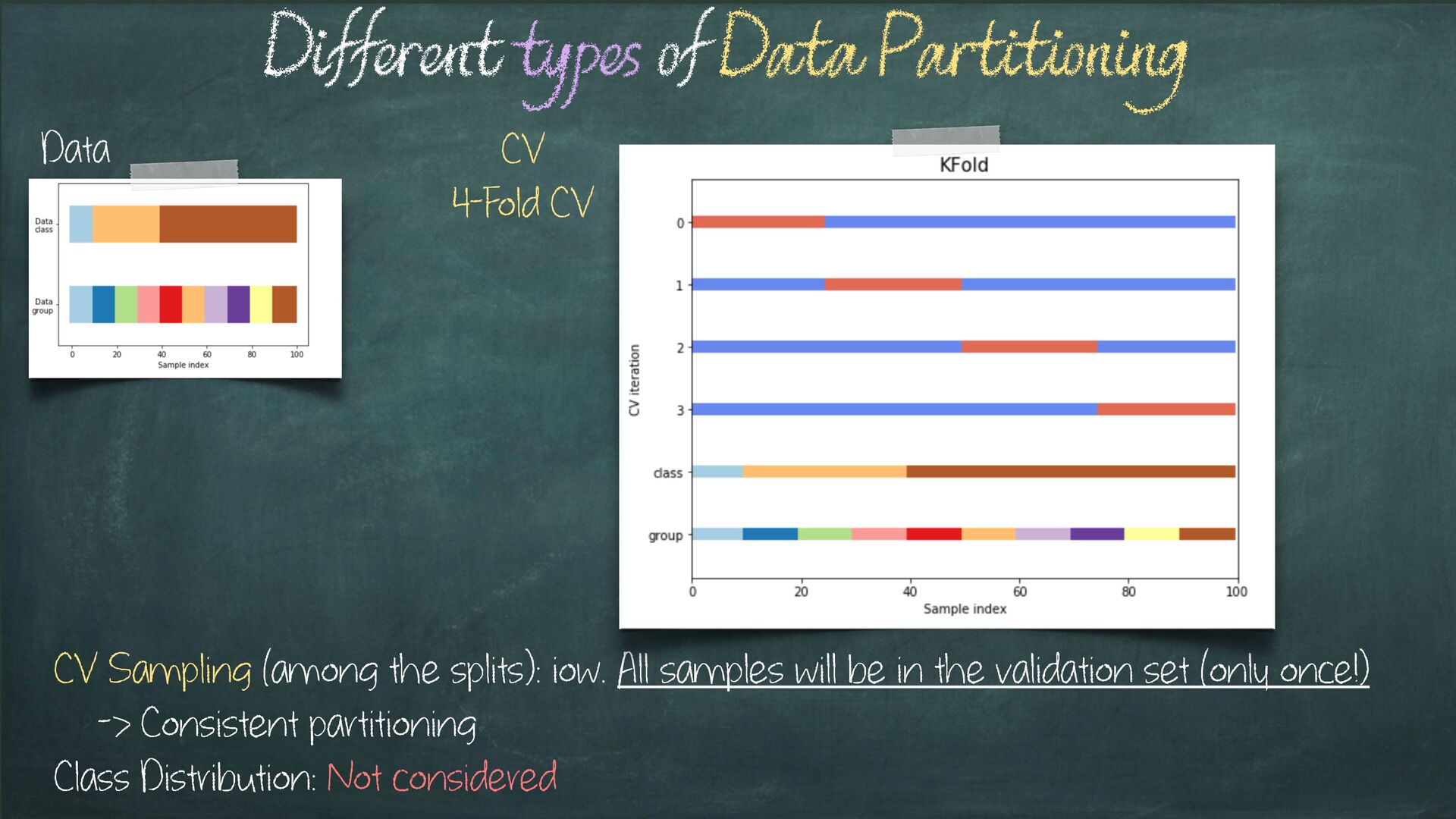
Sampling (among the splits): iow. Sampling w/ Replacement -> Samples are assigned to test partition at random (i.e. 0 or >=1 times) Class Distribution: Not considered
Sampling (for each round): iow. Random but Consistent Partitioning -> All samples will be in the valid. set multiple times but only once for each CV round Class Distribution: Not considered
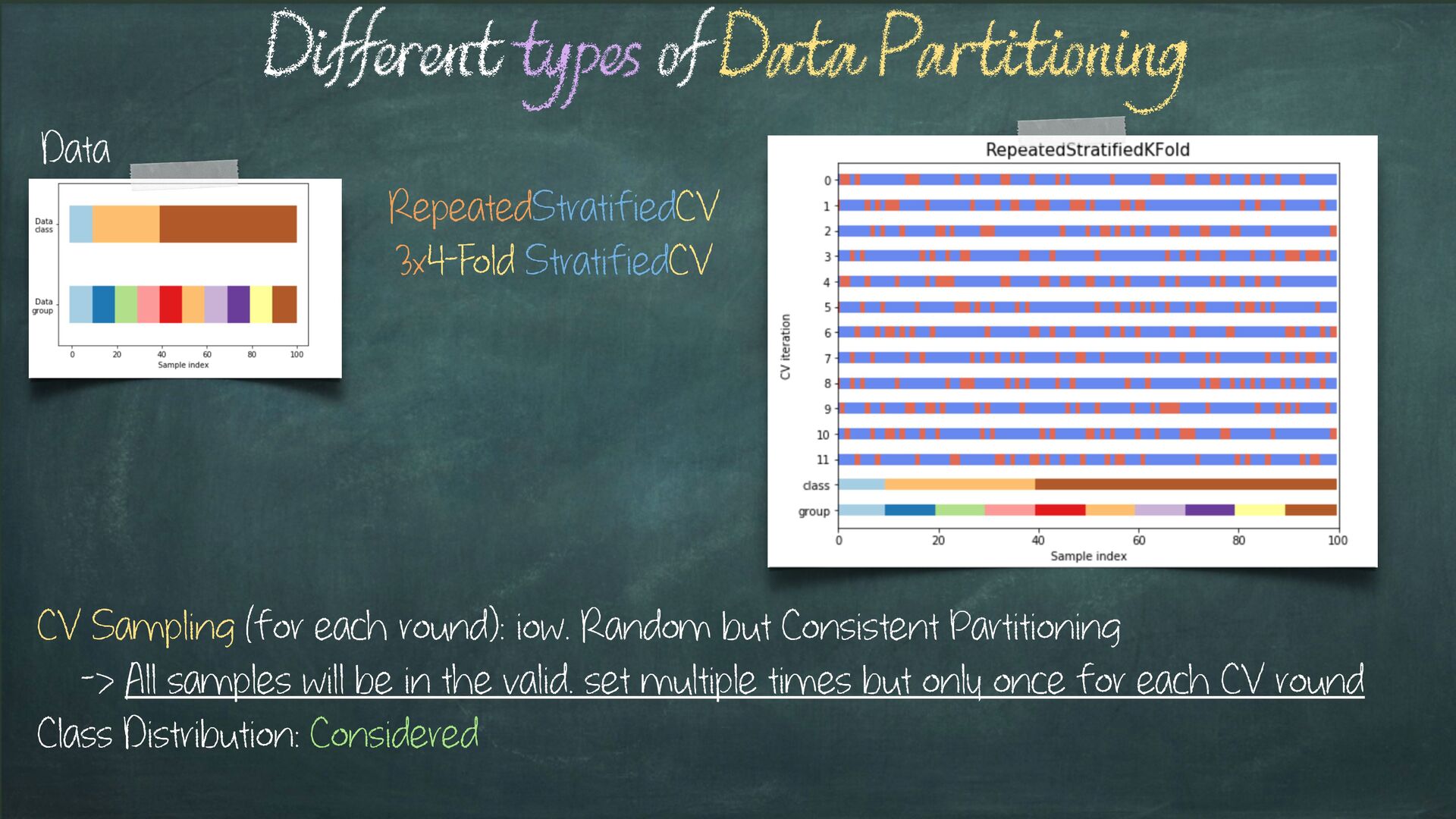
Sampling (for each round): iow. Random but Consistent Partitioning -> All samples will be in the valid. set multiple times but only once for each CV round Class Distribution: Considered
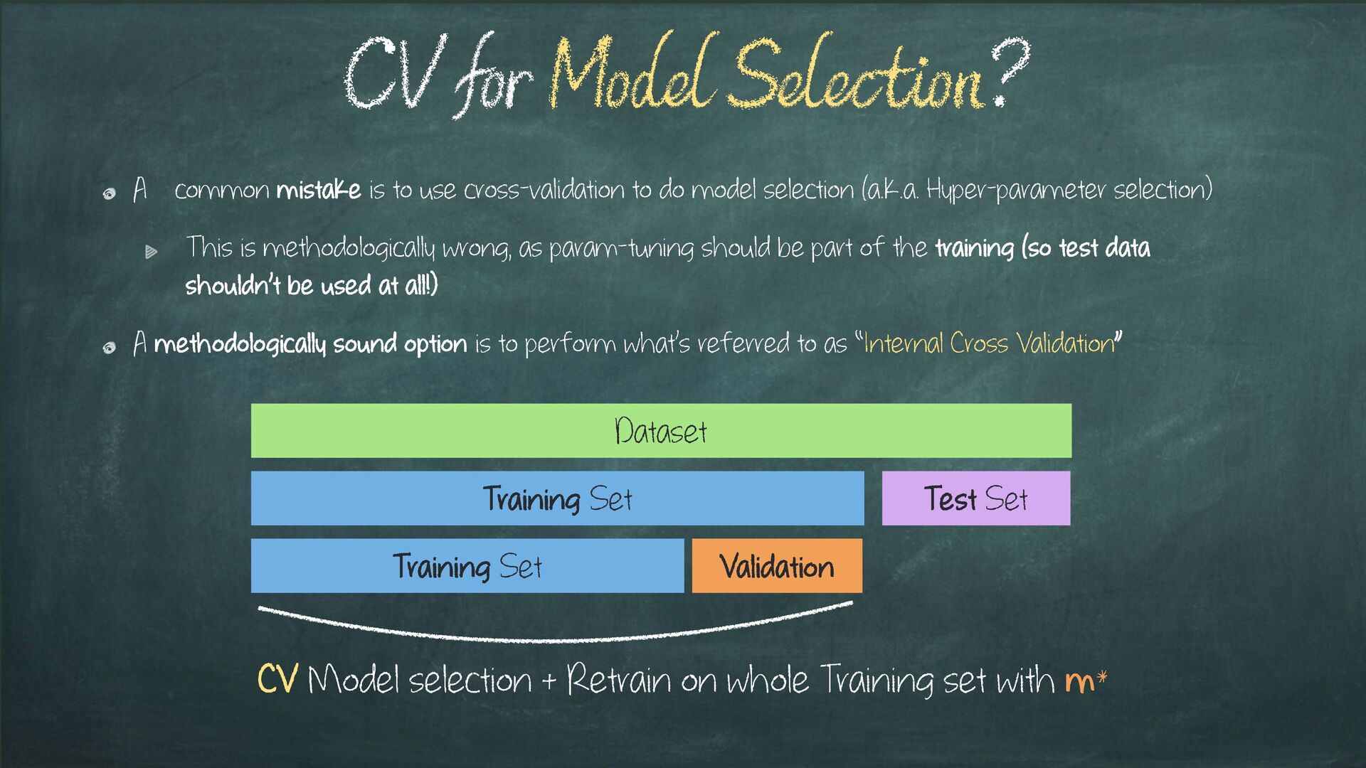
selection (a.k.a. Hyper-parameter selection) This is methodologically wrong, as param-tuning should be part of the training (so test data shouldn’t be used at all!) A methodologically sound option is to perform what’s referred to as “Internal Cross Validation” CV for Model Selection? Dataset Training Set Test Set Training Set Validation CV Model selection + Retrain on whole Training set with m*
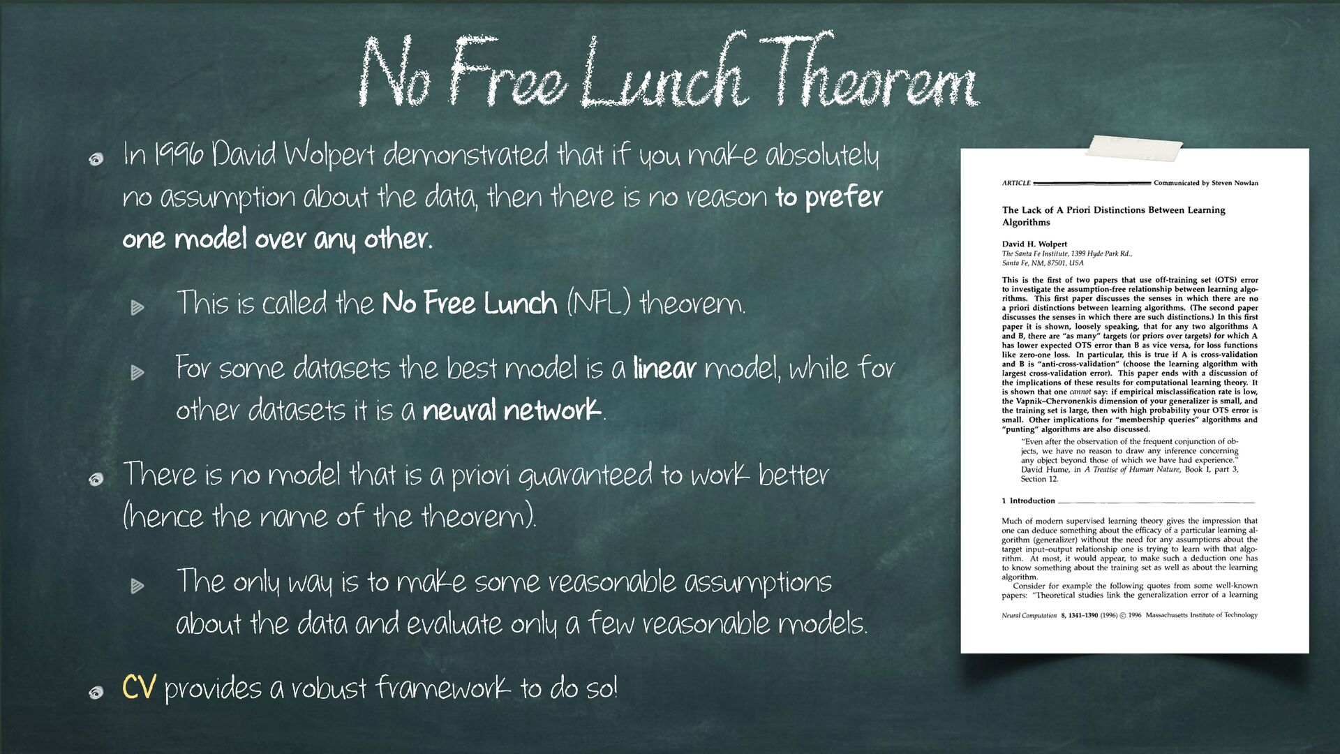
no assumption about the data, then there is no reason to prefer one model over any other. This is called the No Free Lunch (NFL) theorem. For some datasets the best model is a linear model, while for other datasets it is a neural network. There is no model that is a priori guaranteed to work better (hence the name of the theorem). The only way is to make some reasonable assumptions about the data and evaluate only a few reasonable models. CV provides a robust framework to do so! No Free Lunch Theorem
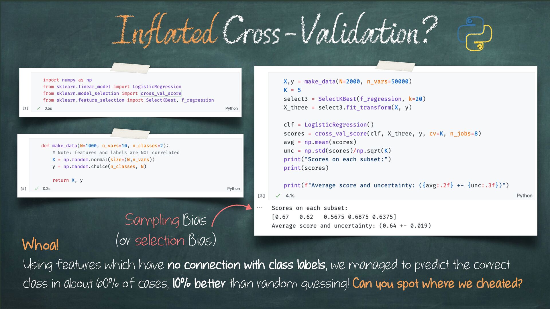
labels, we managed to predict the correct class in about 60% of cases, 10% better than random guessing! Can you spot where we cheated? Whoa! Sampling Bias (or selection Bias)
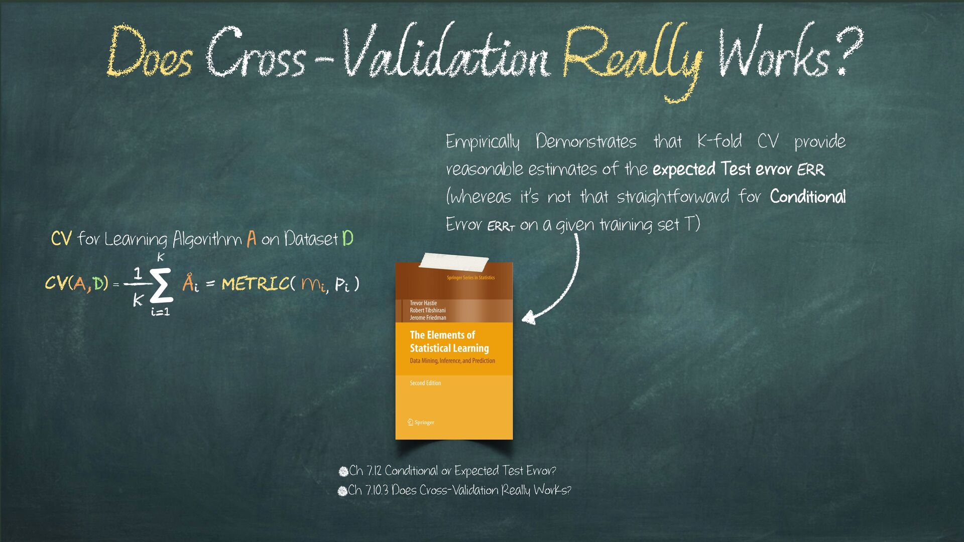
Dataset D Ch 7.12 Conditional or Expected Test Error? Empirically Demonstrates that K-fold CV provide reasonable estimates of the expected Test error Err (whereas it’s not that straightforward for Conditional Error ErrT on a given training set T) Ch 7.10.3 Does Cross-Validation Really Works? CV(A,D) = 1 K Σ K i=1 Åi = metric( mi, Pi )
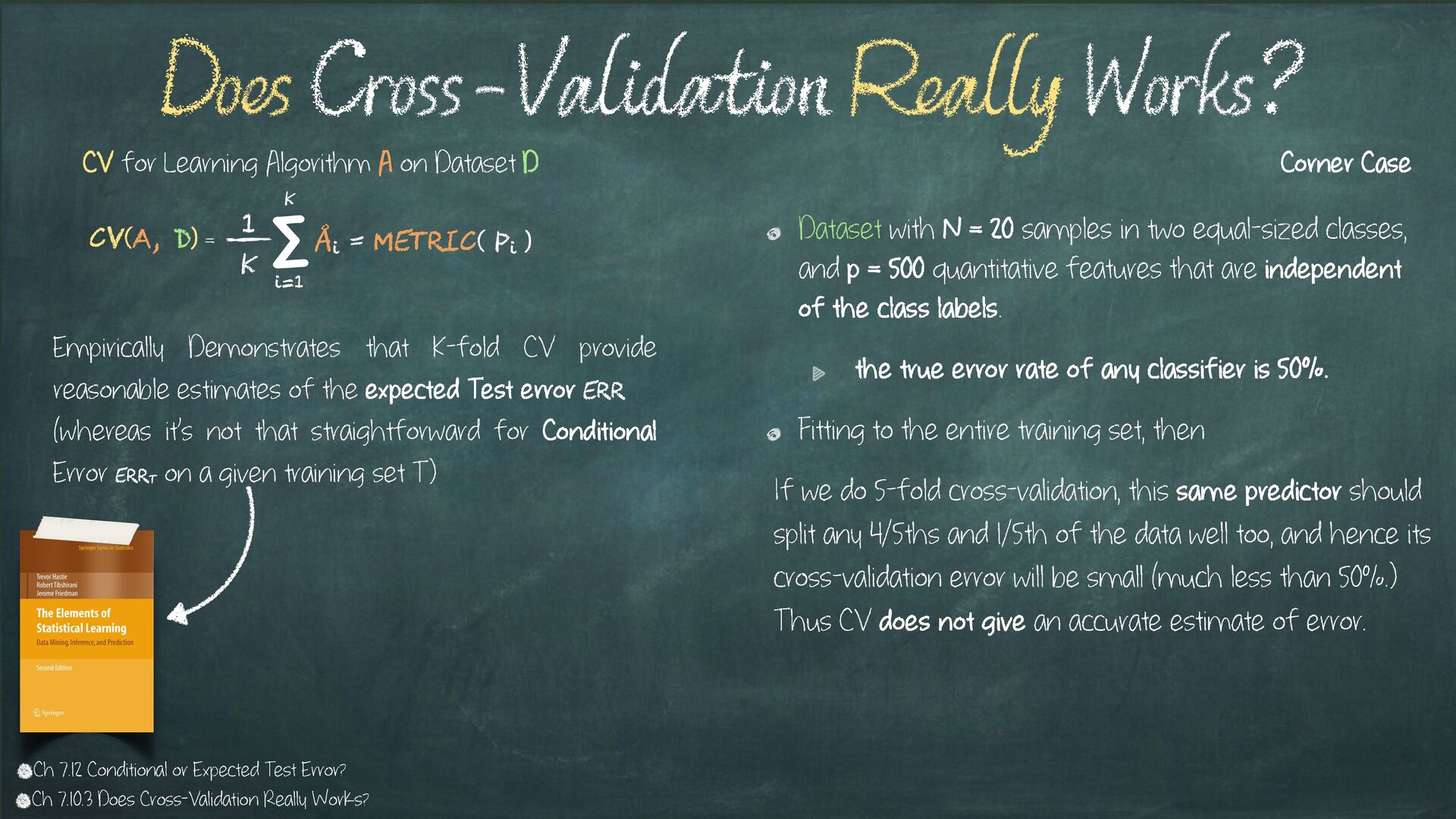
and p = 500 quantitative features that are independent of the class labels. the true error rate of any classifier is 50%. Fitting to the entire training set, then If we do 5-fold cross-validation, this same predictor should split any 4/5ths and 1/5th of the data well too, and hence its cross-validation error will be small (much less than 50%.) Thus CV does not give an accurate estimate of error. Does Cross-Validation Really Works? CV(A, D) = 1 K Σ K i=1 Åi = metric( Pi ) CV for Learning Algorithm A on Dataset D Ch 7.12 Conditional or Expected Test Error? Empirically Demonstrates that K-fold CV provide reasonable estimates of the expected Test error Err (whereas it’s not that straightforward for Conditional Error ErrT on a given training set T) Corner Case Ch 7.10.3 Does Cross-Validation Really Works?
The argument has ignored the fact that in cross-validation, the model must be completely retrained for each fold The Random Labels trick can be a useful sanitisation trick for your CV pipeline Different Performance Avg. Error = 0.5 as it should be! (i.e. Random Guessing) Take Aways
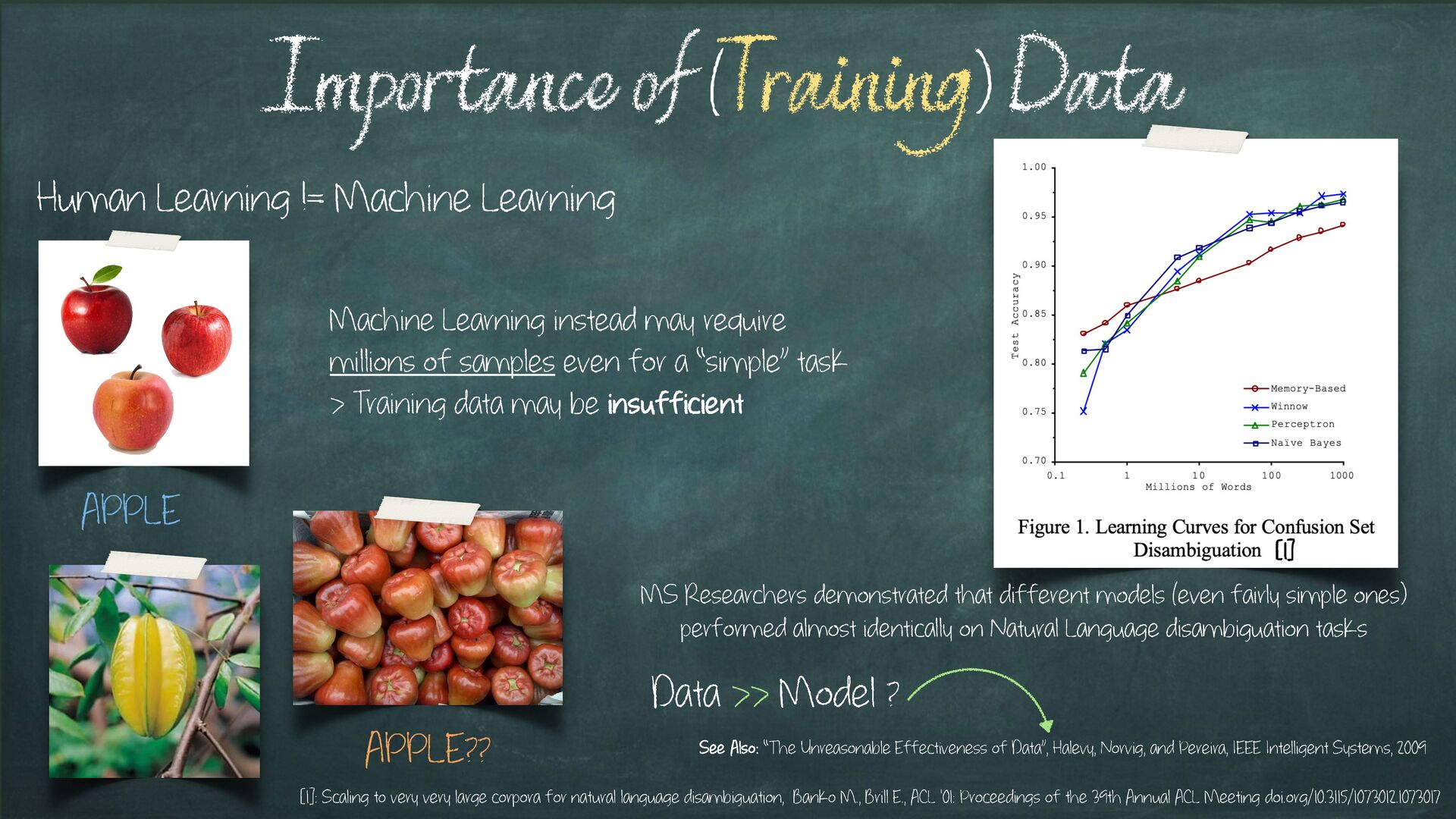
Machine Learning instead may require millions of samples even for a “simple” task > Training data may be insufficient APPLE?? [1]: Scaling to very very large corpora for natural language disambiguation, Banko M., Brill E., ACL '01: Proceedings of the 39th Annual ACL Meeting doi.org/10.3115/1073012.1073017 [1] MS Researchers demonstrated that different models (even fairly simple ones) performed almost identically on Natural Language disambiguation tasks Data >> Model ? See Also: “The Unreasonable Effectiveness of Data”, Halevy, Norvig, and Pereira, IEEE Intelligent Systems, 2009
(B:How) the evaluation plan We now need to establish a tool to interpret the results, e.g. reliable? robust? iow/ We need to deal with the inevitable uncertainty associated with [every] measurement Possible things we could do: Confidence Interval (on a single test set) Bootstrap Confidence Interval on CV statistics Statistic Significance tests e.g. Compare multiple learning algorithms on the same data or multiple datasets How to Interpret Results ?
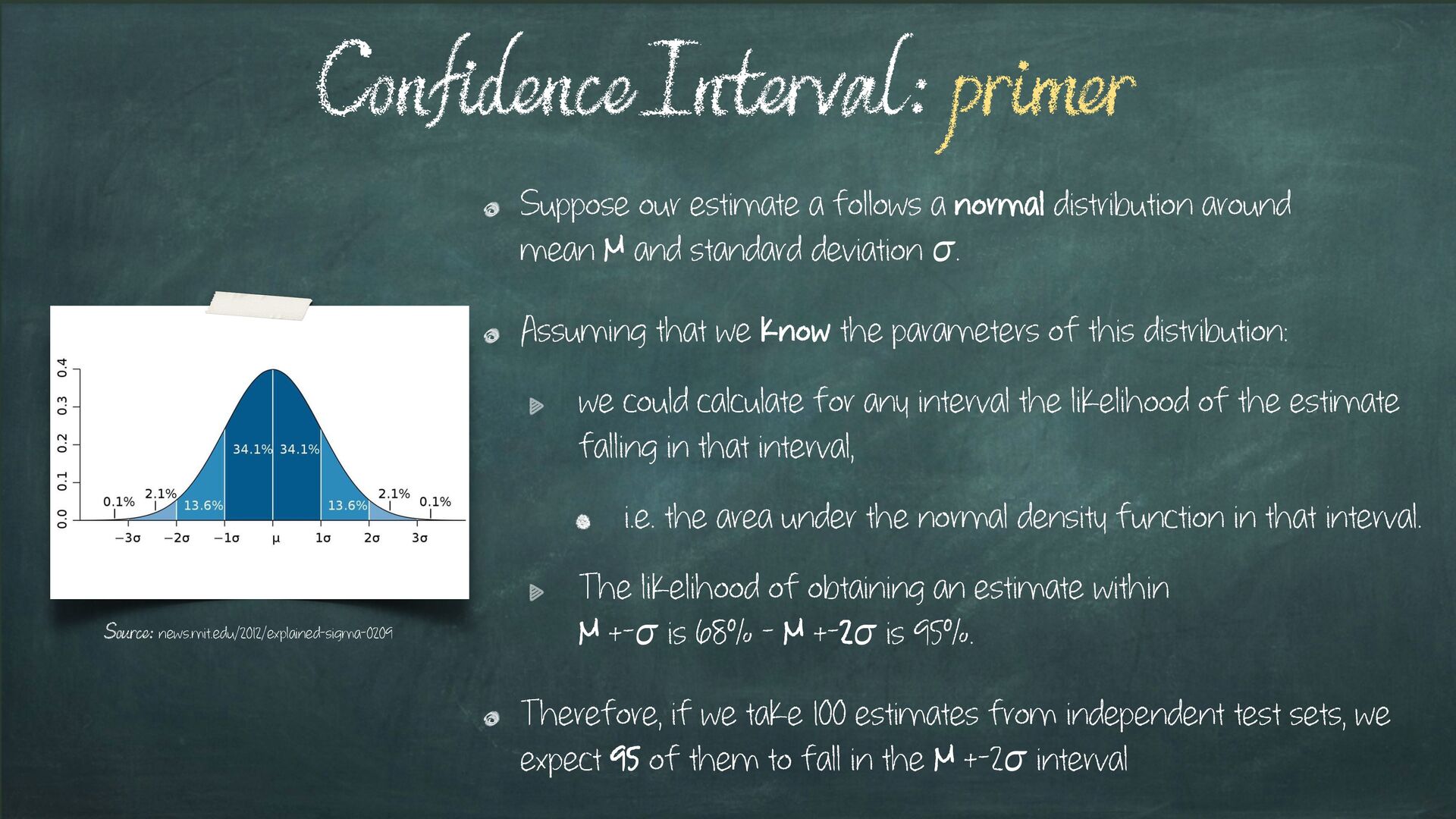
µ and standard deviation . Assuming that we know the parameters of this distribution: we could calculate for any interval the likelihood of the estimate falling in that interval, i.e. the area under the normal density function in that interval. The likelihood of obtaining an estimate within µ +- is 68% - µ +-2 is 95%. Therefore, if we take 100 estimates from independent test sets, we expect 95 of them to fall in the µ +-2 interval Confidence Interval: primer Source: news.mit.edu/2012/explained-sigma-0209
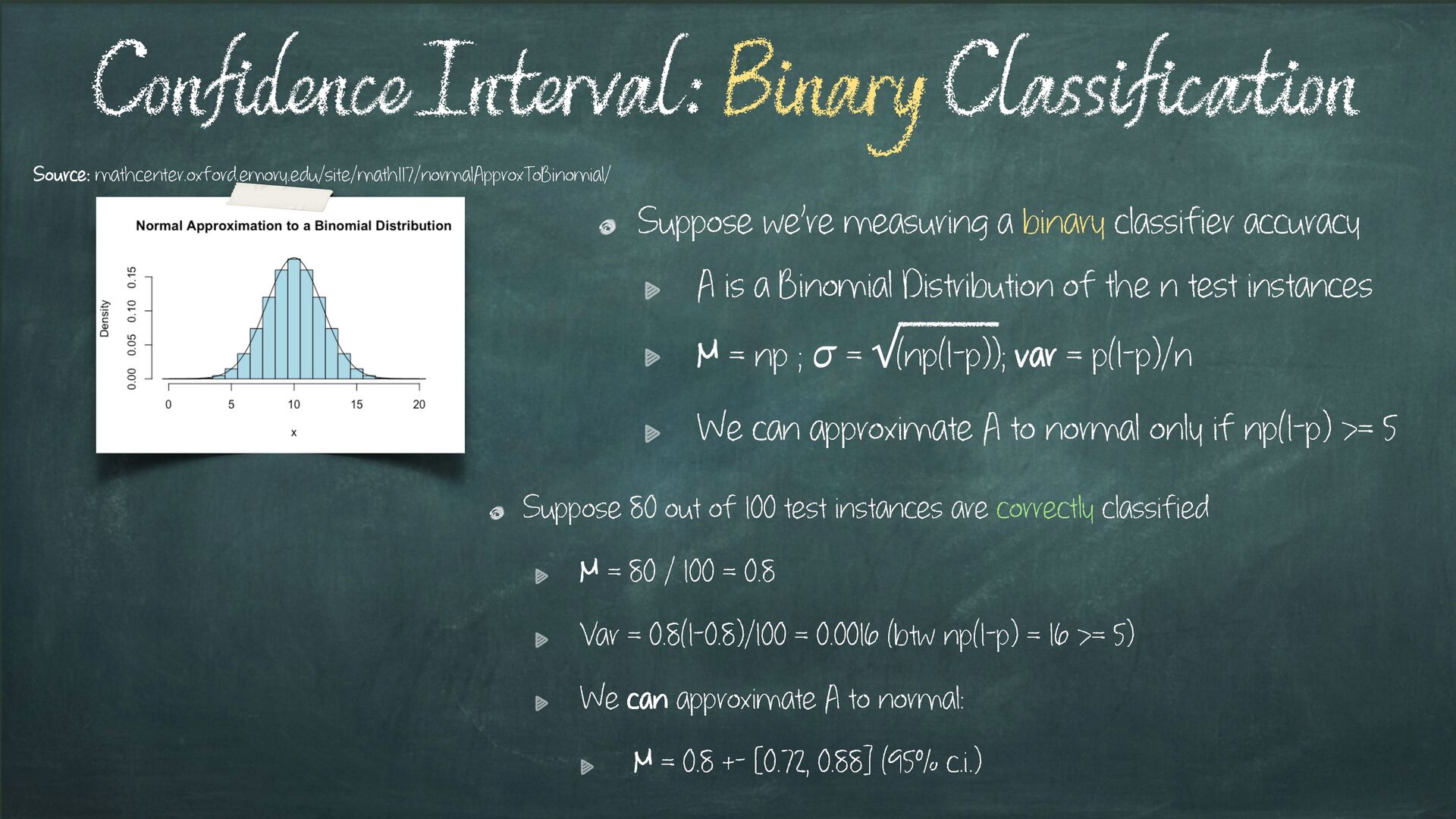
Binomial Distribution of the n test instances µ = np ; = √(np(1-p)); var = p(1-p)/n We can approximate A to normal only if np(1-p) >= 5 Confidence Interval: Binary Classification Source: mathcenter.oxford.emory.edu/site/math117/normalApproxToBinomial/ µ - 2 > 0 and µ + 2 < n np - 2√(np(1-p)) > 0 => np > 2√(np(1-p)) => n2p2 > 4np(1-p) => np > 4(1-p) => np > 4 - 4p. Considering that p in [0, 1], as long as we ensure np > 5 the condition is satisfied!
instances are correctly classified µ = 80 / 100 = 0.8 Var = 0.8(1-0.8)/100 = 0.0016 (btw np(1-p) = 16 >= 5) We can approximate A to normal: µ = 0.8 +- [0.72, 0.88] (95% c.i.) Source: mathcenter.oxford.emory.edu/site/math117/normalApproxToBinomial/ Suppose we’re measuring a binary classifier accuracy A is a Binomial Distribution of the n test instances µ = np ; = √(np(1-p)); var = p(1-p)/n We can approximate A to normal only if np(1-p) >= 5
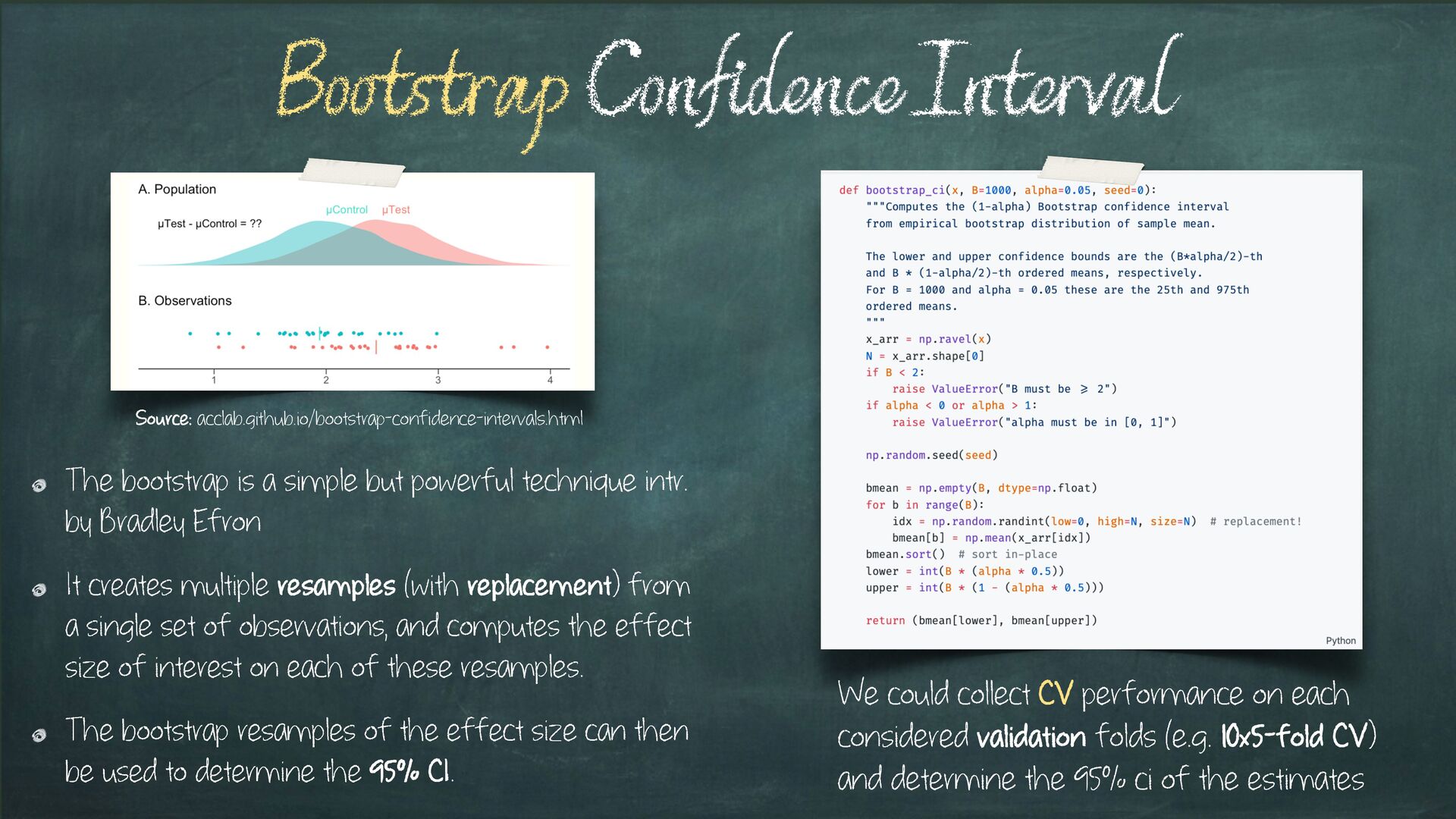
Bradley Efron It creates multiple resamples (with replacement) from a single set of observations, and computes the effect size of interest on each of these resamples. The bootstrap resamples of the effect size can then be used to determine the 95% CI. Bootstrap Confidence Interval Source: acclab.github.io/bootstrap-confidence-intervals.html We could collect CV performance on each considered validation folds (e.g. 10x5-fold CV) and determine the 95% ci of the estimates
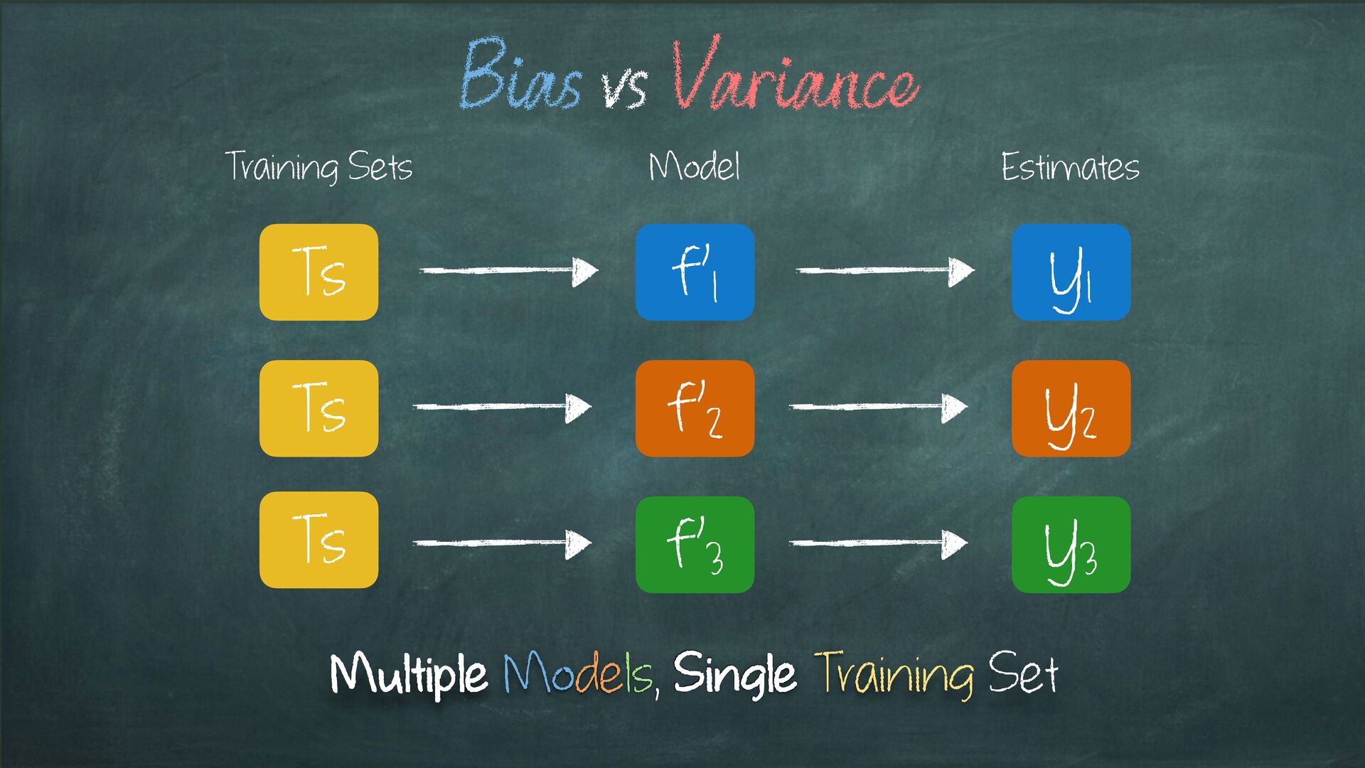
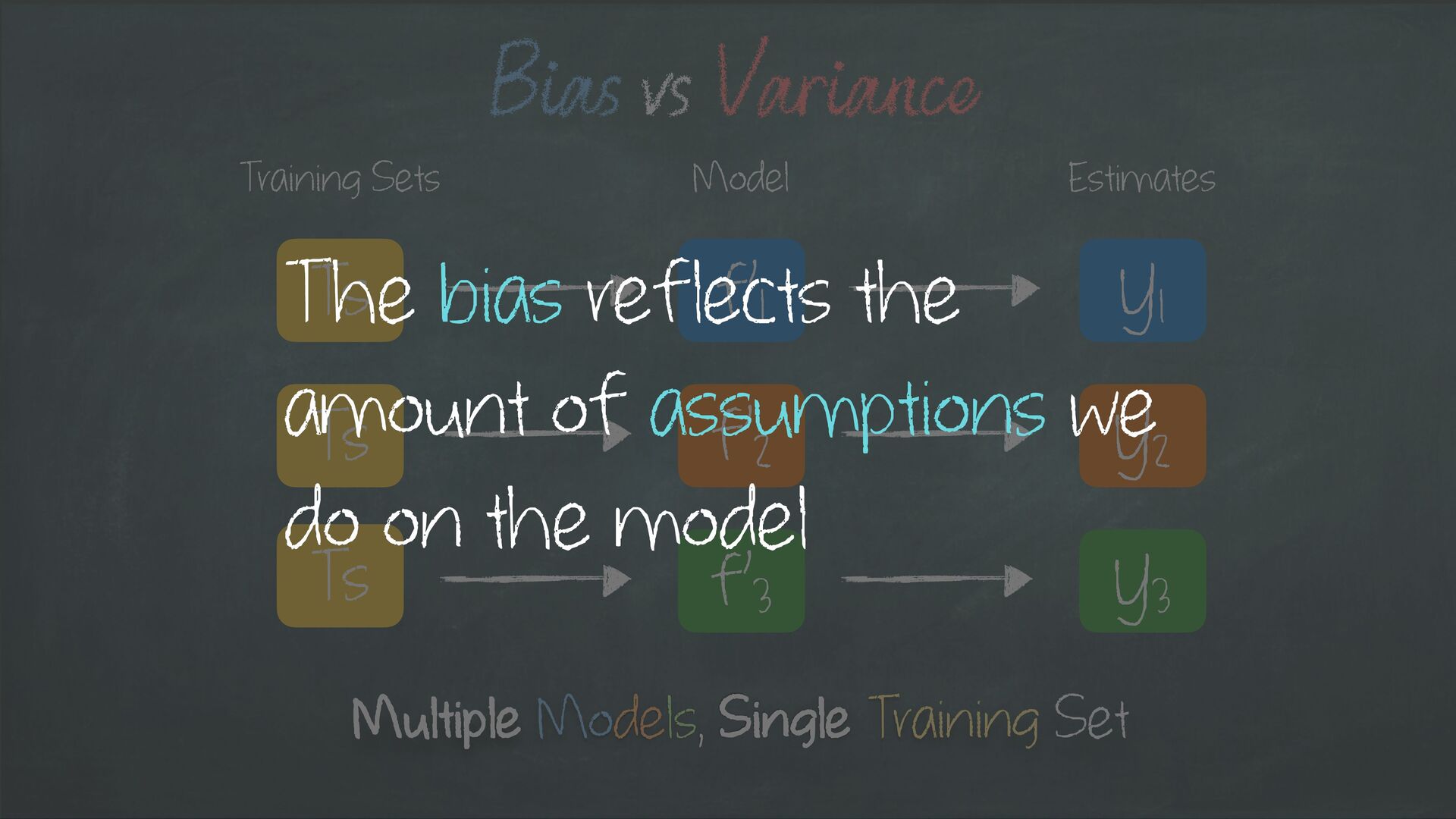
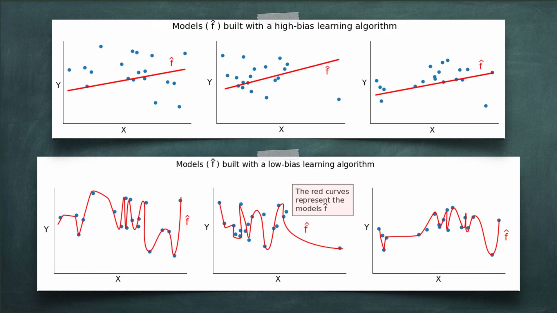
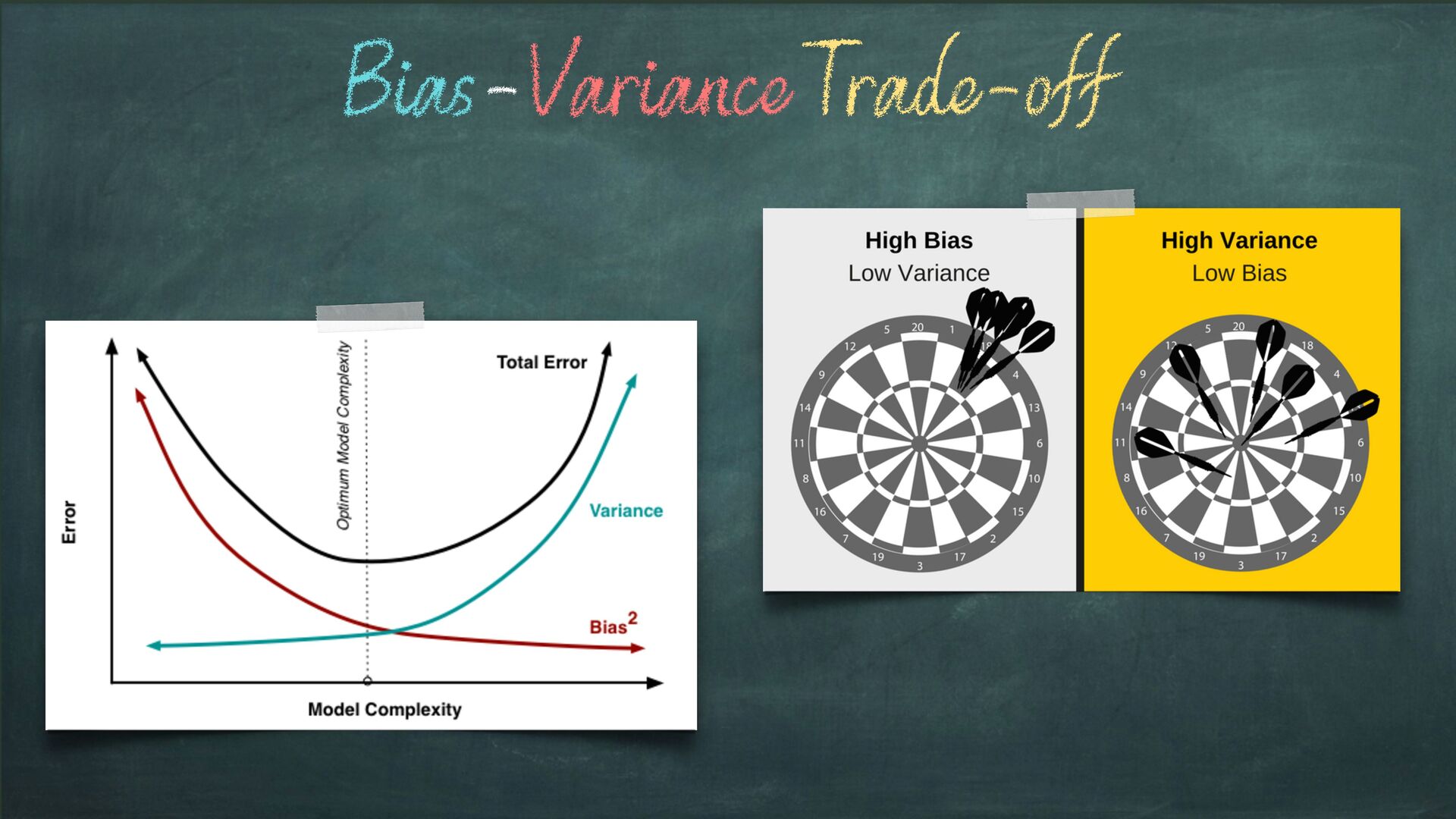
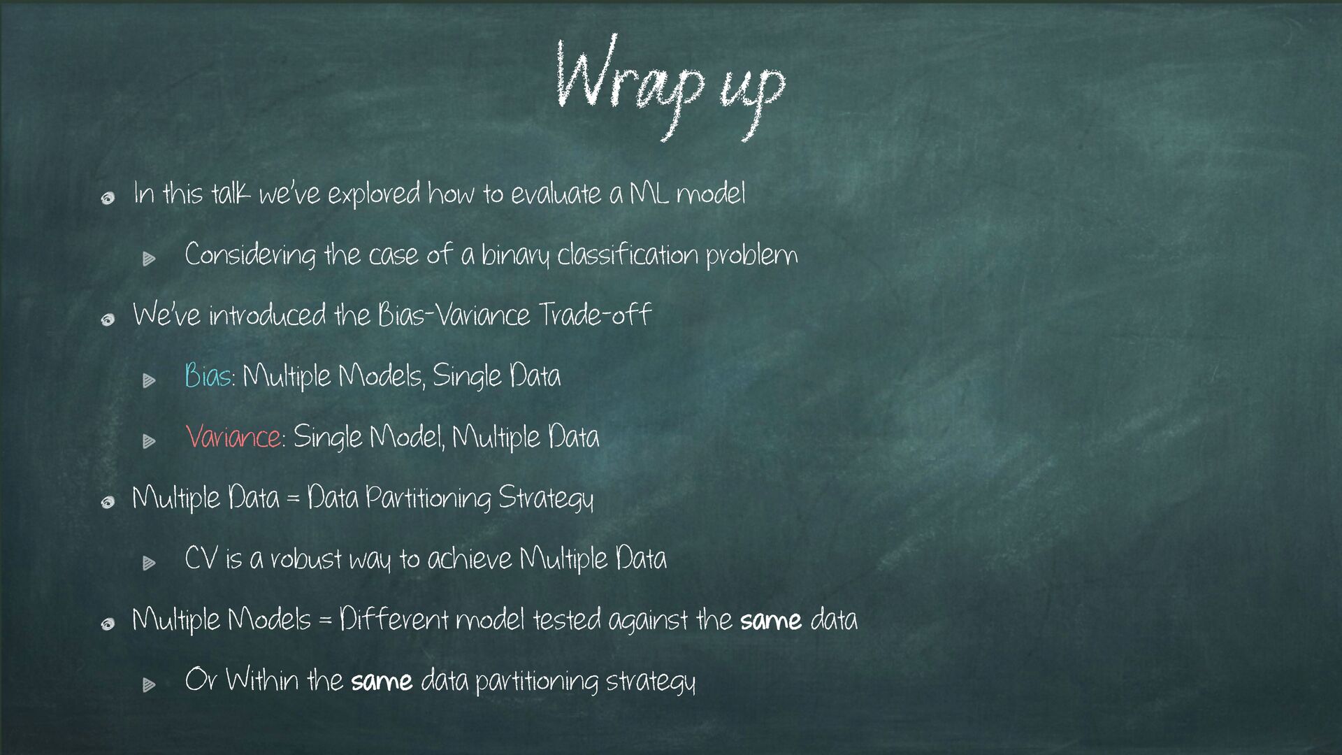
model Considering the case of a binary classification problem We’ve introduced the Bias-Variance Trade-off Bias: Multiple Models, Single Data Variance: Single Model, Multiple Data Multiple Data = Data Partitioning Strategy CV is a robust way to achieve Multiple Data Multiple Models = Different model tested against the same data Or Within the same data partitioning strategy Wrap up
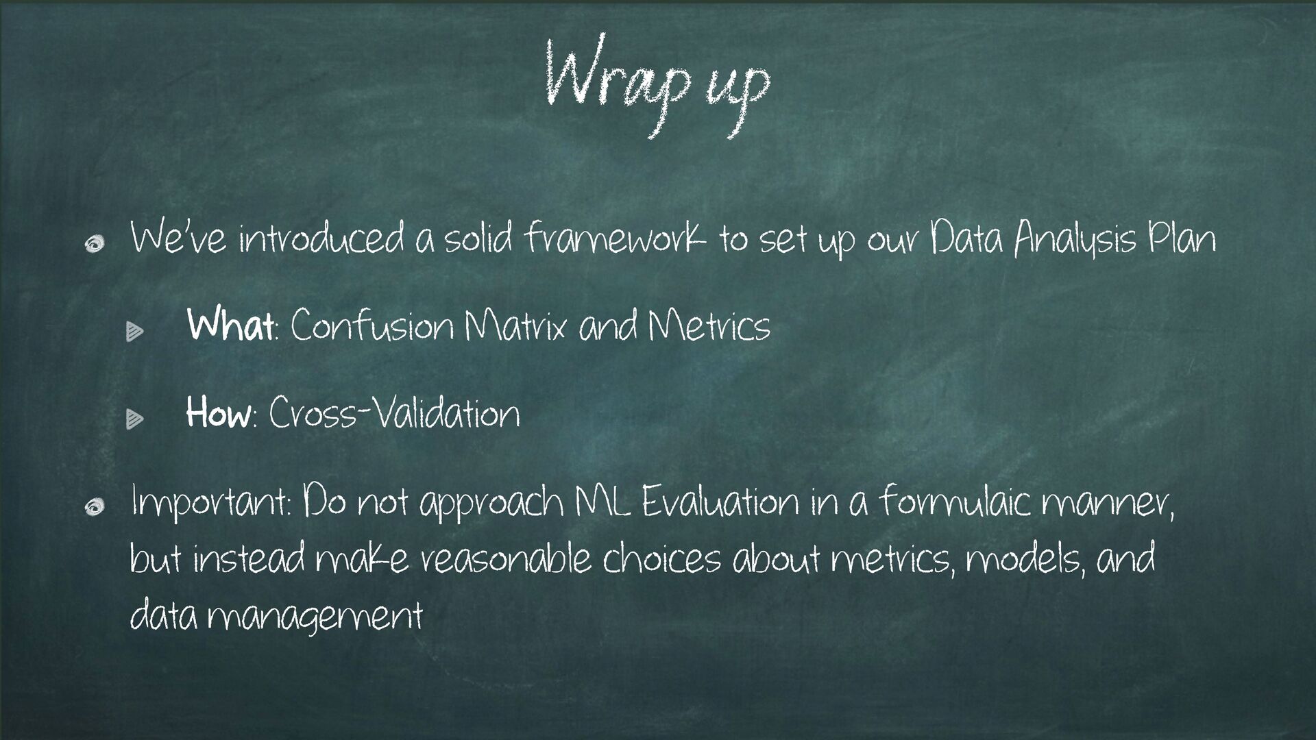
Analysis Plan What: Confusion Matrix and Metrics How: Cross-Validation Important: Do not approach ML Evaluation in a formulaic manner, but instead make reasonable choices about metrics, models, and data management Wrap up
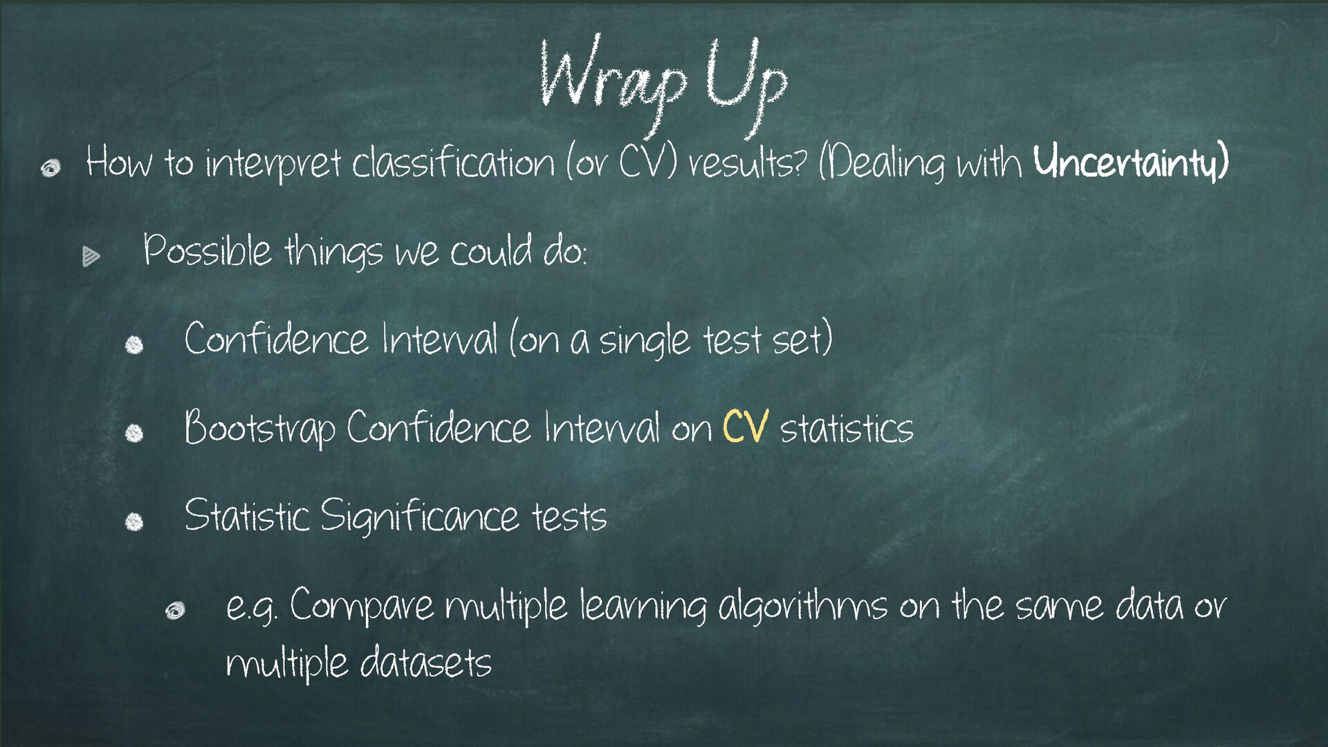
Possible things we could do: Confidence Interval (on a single test set) Bootstrap Confidence Interval on CV statistics Statistic Significance tests e.g. Compare multiple learning algorithms on the same data or multiple datasets Wrap Up
A survey of cross-validation procedures for model selection DOI: 10.1214/09-SS054 [Article] IID Violation and Robust Standard Errors https://stat-analysis.netlify.app/the-iid-violation-and-robust-standard- errors.html Non i.i.d. Data and Cross Validation: https://inria.github.io/scikit-learn-mooc/python_scripts/ cross_validation_time.html References and Further Readings References
![Evaluating Machine Learning Models @leriomaggio Valerio Maggio, PhD [email protected]](https://files.speakerdeck.com/presentations/f5b3e2e344874734bdb686038e853b4e/slide_0.jpg)
![ML Experiment: Research Question (RQ); Learning Algorithm (A, m); Dataset[s]](https://files.speakerdeck.com/presentations/f5b3e2e344874734bdb686038e853b4e/slide_8.jpg)
![Is F-Measure (F1) a Good Idea? [1]: “Machine Learning. The](https://files.speakerdeck.com/presentations/f5b3e2e344874734bdb686038e853b4e/slide_49.jpg)
![[Article] Why every statistician should know about cross-validation (https://robjhyndman.com/hyndsight/crossvalidation/) [Paper]](https://files.speakerdeck.com/presentations/f5b3e2e344874734bdb686038e853b4e/slide_87.jpg)
![Thank you very much for your kind attention @leriomaggio [email protected]](https://files.speakerdeck.com/presentations/f5b3e2e344874734bdb686038e853b4e/slide_88.jpg)