QQ

Plagiarized manuscript

Transcript

1. Abstract—In recent year, the awareness of environmental protection has made the power dispatch model on longer purely economical-oriented. This paper presents a modified particle swarm optimization (MPSO) approach to solve the Unit Commitment (UC) problem for 24 hours at the maximum profit in the power and carbon market. Solving the UC problem for 24 hours in the interconnected power network that is comprised of three independent areas to approach the best dispatching strategy. The UC problem must satisfy the constraints such as the load demand, generating limits, minimum up/down time and ramp rate limits, and also involves determining the limits of power flow, buses voltage and transmission line capacity. The Independent Power Producer (IPP) can obtain the maximum profit by the power and carbon trading amount and calculating power wheeling expense based on the 24-hour power and carbon forecasting trading data. Furthermore, it can also be assessed the basis of participating in the trading market or not. keywords—Unit Commitment, Multiple Particle Swarm Optimization, Emission, Carbon Trading, Carbon market I. INTRODUCTION From a financial and commodity markets perspective, wholesale electricity prices can generally be viewed as the result of investors having created real options upon various underlying primary fuel commodities such as gas, oil or coal. Although a substantial amount of electricity is generated from hydro and nuclear sources in various parts of the world, the dominant production process is still the thermal conversion of fossil fuels such as gas, oil and coal. Thus, as electricity is often traded on exchanges close to an hour before it is needed, in this short term, the variable cost of power generation is essentially just the cost of the fuel. Even in power systems with a substantial amount of hydro and nuclear, it is the fossil fuel plant that often sets the market prices. Depending upon the age and technology of the generating plant, in general, around a half of the energy content of the primary fuel gets converted into electricity. It follows from this, that with knowledge of the spot and futures market prices for primary fuels, and relatively well-known efficiency ratings for individual power plants on the system, the short-run marginal cost of each power plant on the system can be reasonably well estimated as a simple conversion of the fuel price. In practice, however, whilst this fundamental concept is valid, its application has many complications [1]. In this market structure, the independent power producers (IPPs) have to deal with several complex issues The Authors are with the Department of Electrical Engineering, National Sun Yat-Sen University, Kaohsiung 80424, Taiwan. (e-mail: D953010011@student.nsysu.edu.tw). arising from uncertainties in spot market prices, and technical constraints which need to be considered while scheduling generation and trading for the next day. In addition to finding dispatch and unit commitment decisions while maximizing its profit, their scheduling models should include trading decisions like spot-market buy and sell [2]. The model proposed in this paper build on the combined bilateral contract and spot market formulation, and help generators in deciding on when these commitments could be beneficial. The other objective of this paper is to investigate an influence of emission constraints on generation scheduling. The motivation for this objective comes from the efforts to reduce negative trends in a climate change. One of the major international instruments to address this problem is the Kyoto Protocol. To help developed countries achieve parts of their emission reduction commitments, Kyoto Protocol includes three market-based mechanisms, one of them being emissions trading. Since electricity sector is one of the major sources of CO2 emissions, under framework of Kyoto Protocol each country decides on the allocation of its portion of permissions and how much will be allocated to the energy sector. This means that electricity market price will be affected by the scheme as electricity produces seek to pass their additional cost to consumers. Furthermore, emission caps will have affect on decisions of generating companies on how much and when to produce in order to use their allocations effectively [3]. Analysis in [4] looks at the problem of SOx emissions, with the formulation that incorporates these constants into an objective function. Lagrange relaxation in a combination with Dantzig-Wolfe decomposition has been applied in [5] to investigate long term security constrained UC, while a combination with evolutionary programming has been suggested in [6] for analysis of profit maximization UC. Formulations of emission functions for different types of pollutants (such as CO2 , SO2 and NOx ) are discussed for various generating units in [7]. In contrast to the above mentioned work that considers only caps on emission allowances, the goal of this paper is to investigate possible influences of an emission and power trading mechanism on decisions of generators. In the past few decades, many stochastic optimization methods have been developed, such as Genetic Algorithms (GA), Evolutionary Programming (EP), Evolution Strategies (ES), Immune Algorithm (IA), particle swarm optimization (PSO) and Simulated Annealing (SA) [15-17]. In this paper, a modified particle swarm optimization algorithm for UC problem with carbon trading is proposed for practical application. Assessment of Power Market for Carbon Trading by Modified Particle Swarm Optimization Whei-Min Lin, Member, IEEE, Kai-Hung Lu, Chia-Sheng Tu and Chih-Ming Hong Proceedings of the International MultiConference of Engineers and Computer Scientists 2012 Vol II, IMECS 2012, March 14 - 16, 2012, Hong Kong ISBN: 978-988-19251-9-0 ISSN: 2078-0958 (Print); ISSN: 2078-0966 (Online) IMECS 2012
2. II. EMISSION FUNCTION This paper presents a short-term generation scheduling model applicable to independent power producers participating in electricity power and carbon markets to find their maximal profit under direct bilateral contracts. It has an unrestricted option to participate in power and carbon market as a buyer and/or a seller. The following derivation of the emissions function is discussed in [8]. In general, CO2 emissions are related to the consumed amount of fuel, and therefore can be expressed based on the following incremental heat rate or Input/Output (I/O) characteristics, 2 1 2 3 ( ( )) ( ) ( ) i Gi i i Gi i Gi H P t k k P t k P t = + + (1) Therefore, the emission function ( ( )) i i EC P t of generator i can be defined as : 2 1 2 3 ( ( )) ( ( ) ( )) i ei Gi i i Gi i Gi EC P t e k k P t k P t = + + (2) where ki1 , ki2 and ki3 are heat rate coefficients and eei is an emission coefficient for each generator i. As the value of coefficient eei depends on a type of a generating unit, as well as on a quality of the used fuel, its value needs to be estimated or calculated in a way that accounts for these variations. A practical way to determine the value of this emission coefficient eei is to base its calculations on the value of emissions that the generator has to compute following a procedure outlined in measurement and report mechanism directives [9]. These documents define that combustion emissions for generator i are calculated as, ( ) ( ) i i i i i ER t fuel t net calorific value emission factor oxidation factor = ⋅ ⋅ ⋅ (3) The above reporting and monitoring of CO2 emissions calculation is based on a measurement of the amount of fuel (in t or Nm3) consumed by generating unit i during a monitoring period. Net calorific valuei and emission factori depend on the particular type of a fuel used, and have to be regularly measured. Emission factor is based on a carbon content of a fuel, and is expressed as tCO2 /TJ, while net calorific value is expressed in TJ/t or TJ/m3. Finally, oxidation factori accounts for the fact that a portion of carbon content remains unburned or partly oxidized and is therefore not emitted into the atmosphere. Now, emission coefficient eei used in (2) can be calculated by matching a value of emissions function (2) and a reported value defined by (3), so that, 2 1 2 3 2 1 2 3 ( ( )) ( ( ) ( )) ( ) ( ( ) ( )) i Gi ei i i Gi i Gi i i i Gi i Gi EC P t e k k P t k P t ER t k k P t k P t = + + = + + (4) The above value can then be used by a generator to define emission function (2). It is interesting to note here that the true fuel cost function, FCi (PGi (t)), of generator i is also related to the incremental heat rate of (1), so that, 2 1 2 3 ( ( )) ( ( ) ( )) Gi i i i Gi i Gi fi P t FC p k k P t k P t = + + (5) Where pfi is the fuel price. In that case, each generator will be allowed to submit its offer function, and only one parameter – overall emission coefficient ei - that will be used to calculate the emissions function (2), 2 1 2 3 ( ( )) ( ( ) ( )) fi fi i ei Gi i i Gi i Gi i ei ei i i i EC P t e k k P t k P t FC e e FC p p e FC = + + = × = × = × (6) This paper assumes the above approach that coefficients of the emission function, ECi (PGi (t)), submitted by generator i are related to the offer function, FCi (PGi (t)), as defined by (6) [3]. III. PROBLEM FORMULATION FOR PRICE-BASED UC WITH CARBON TRADING The proposed price-based unit commitment problem with carbon trading can be mathematically expressed as the following optimization problem. A. Objective function: In this framework the purpose of the objective function is to be maximal profit: IPP's profit= Revenue-Cost where Revenue= (spot market sell) + (carbon market sell) + (bilateral power sell) Cost= (spot market buy) + (carbon market buy) + (unit operating costs) + (start-up costs) Defining the new UC problem involves changing the objective function from cost minimization to profit maximization. The objective function can be mathematically expressed as the following equation: Max profit = Revenue -Cost (7) ( ) t t t t t t Revenue us PS cs ES BC CP = + × × + × (8) ) ( it t t t t it Cost ub PB cb EB FC ST = + + × × + (9) or Min Payment=Cost-Revenue (10) where Profit : Profit of the IPP, $. ust : Power sale price by IPP to spot market, $/MWh. cst : Carbon sale price by IPP to carbon market, $/kg. ubt : Power purchase price by IPP from spot market, $/MWh. cbt : Carbon purchase price by IPP from carbon market, $/kg. PSt : Power sale by IPP to spot market, MWh. ESt : Carbon sale by IPP to spot market, kg. PBt : Power purchase by IPP from spot market, MWh. EBt : Carbon purchase by IPP from carbon market, kg. BCt : Bilateral contracted demand, MWh. CPt : Bilateral contracted power selling price, $/MWh. STit : start-up cost of unit i at t-th hour. B. Constraints: (1). Power balance constraints 1 1 ( ) ( ) G i T G t t t i D t Rt t P PB PS P P = = + − + ≤ ∑ ∑ (11) PDt : Demand at t-th hour PRt : Spinning reserve at t-th hour (2). Minimum up-time and down-time These minimum uptime and minimum downtime constraints reduce the opportunities to change the status of the unit and can have a profound impact on the optimal schedule. Ton (i)≥ Tiu Toff (i)≥ Tid Ton (i): the continual up-time of unit i. Toff (i): the continual down-time of unit i. Tiu : minimal up-time of unit i. (3). Maximum and minimum output limits The power output of any generator should not exceed its rating nor should it be below that necessary for stable boiler Proceedings of the International MultiConference of Engineers and Computer Scientists 2012 Vol II, IMECS 2012, March 14 - 16, 2012, Hong Kong ISBN: 978-988-19251-9-0 ISSN: 2078-0958 (Print); ISSN: 2078-0966 (Online) IMECS 2012
3. operation. Thus, the generations are restricted to lie within given minimum and maximum limits. Pmin ≤PGi (t)≤Pmax (12) Pmin : the minimum generation limits of unit i. Pmax : the maximum generation limits of unit i. (4). Ramp rate limits Starting up or shutting down a thermal generating unit or even increasing or decreasing its output by more than a small amount causes considerable mechanical stress in the prime mover. ( ) ( 1) as generation increases Gi Gi i P t P t UR − − ≤ (13) ( 1) ( ) as generation decreases Gi Gi i P t P t DR − − ≤ (14) URi : ramp-up rate limit of unit i. DRi : ramp-down rate limit of unit i. (5). Emission limits max 1 1 ( ) ( ( ) ) T G t t Gi t i t EC EC P ES EB = = ≥ + − ∑ ∑ (6). Trading limits 0≤PSt ≤ PSt max (15) 0≤ ESt ≤ ESt max (16) 0≤ PBt ≤ PBt max (17) 0≤ EBt ≤ EBt max (18) PSt max: Max power sold allowances, MWh. ESt max: Max carbon sold allowances, kg. PBt max: Max power bought allowances, MWh. EBt max: Max carbon bought allowances, kg. IV. MODIFIED PARTICLE SWARM OPTIMIZATION A. Basic PSO PSO, as a population-based algorithm, exploits a population of individuals to probe promising regions of the search space. The population is called a swarm and the individuals, particles. As the swarm iterates, the fitness of the global best solution improves (decreases for minimization problem). It is expected to happen that all particles being influenced by the global best eventually approach the global best. If the fitness does not improve despite however many runs the PSO is iterated, then convergence has been achieved. In the pioneering work of Kennedy and Eberhart in 1995, the particle position and velocity is defined by: ) _ ( ) _ ( ] ][ [ ] ][ [ 2 2 ] ][ [ ] ][ [ 1 1 ] ][ [ 1 ] ][ [ k j i k j i k j i k j i k j i k j i X Gbest X rand C X Lbest X rand C V V − ⋅ ⋅ + − ⋅ ⋅ + = + (19) 1 ] ][ [ ] ][ [ 1 ] ][ [ + + + = k j i k j i k j i V X X Where: [i],[j] Population number and particles number. k j i V ] ][ [ Velocity of the particle in the kth iteration. k j i X ] ][ [ Position of the particle in the kth iteration. k j i Lbest X ] ][ [ _ Ith fitness best in the kth iteration. k j i Gbest X ] ][ [ _ Population global best in the kth iteration. C1 , C2 Cognitive and Social component, respectively: they influence how much the particle’s personal best and the global best (respectively) influence its movements. rand1 , rand2 Uniform random numbers between 0 and 1. B. Modified PSO A weight factor, ωk , was added to the previous velocity of the particle. This allows control on the mechanism responsible for the velocities magnitude, which fosters the danger of swarm explosion and divergence, or fast convergence and being trapped in local minima. Thus, equation (19) can be re-written including the weight factor, ωk . ) _ ( ) _ ( ] ][ [ ] ][ [ 2 2 ] ][ [ ] ][ [ 1 1 ] ][ [ 1 ] ][ [ k j i k j i k j i k j i k j i k k j i X Gbest X rand C X Lbest X rand C V V − ⋅ ⋅ + − ⋅ ⋅ + ∗ = + ω (20) 1 ] ][ [ ] ][ [ 1 ] ][ [ + + + = k j i k j i k j i V X X The second challenge is to find a feasible weight factor that prevents prematurely because it affects the convergence and the ability of the swarm to find the optimum. A suitable value of ωk provides the desired balance between the global and local exploration ability of the swarm and, consequently, improves the effectiveness of the algorithm. At the beginning, a large inertial weight is better because it gives priority to global exploration of the search space. It can be gradually decreased so as to obtain refined solutions. To introduce chaotic behavior, the iterator called Logistic Map is defined by the following equation: ) 1 ( 1 1 − − − ⋅ = k k k f f f µ (21) Where µ is a control parameter and has a real value between 0 and 4. Despite the apparent simplicity of the equation, the solution exhibits a rich variety of behaviors. The value of µ determines whether fk stabilizes at a constant size, oscillates between a limited sequence of sizes, or behaves chaotically in an unpredictable pattern. And also the behavior of the system is sensitive to initial values of fk . Equation (20) displays chaotic dynamics when µ=4.0 and { } 0 . 1 , 75 . 0 , 5 . 0 , 25 . 0 , 0 0 ∉ f [18]. After some tests, the value chosen for ω0 , µ and f0 are 3.5, 4.0 and 0.65, respectively. Therefore, the weight inertial factor is calculated in every kth iteration as: ( ) ) ( log 1 2 0 k k f k ⋅       + = ω ω (22) V. SIMULATION AND RESULTS Two case studies are carried out to show this: Case 1 — When all generators have no power and carbon trades and sufficient carbon emission allowances so that generation scheduling is not affected by market clearing. The objective of this case is to find the minimal costs. Case 2 — When both power and carbon trades affect generation scheduling. The IPP must meet its bilateral contracts and commit its carbon emission allowances. The objective of this case is to find the maximal profits. System data [3]: The Cases simulations test runs for 5 unit systems. The resulting search space is vaster. The system data and load data are given in Table 1 and 2. As for emission coefficients, they are assumed as given in table 3. The proposed method is used fixed parameters. Table 1：System data for the 5-unit. Pmin (MWh) Pmax (MWh) a ($/h) b ($/MWh) C ($/MW2h) Min up Time (h) Min down Time (h) Cold Start Hr (h) Hot Start Cost ($) Cold Start Cost ($) Initial Status (h) Unit1 150 455 0.00048 16.19 1000 8 8 8 4500 9000 8 Unit2 20 130 0.002 16.6 700 5 5 5 550 1100 -5 Unit3 20 130 0.00211 16.5 680 5 5 5 560 1120 -5 Unit4 20 80 0.00712 22.26 370 3 3 3 170 340 -3 Unit5 55 55 0.00413 25.92 660 1 1 1 30 60 -1 Proceedings of the International MultiConference of Engineers and Computer Scientists 2012 Vol II, IMECS 2012, March 14 - 16, 2012, Hong Kong ISBN: 978-988-19251-9-0 ISSN: 2078-0958 (Print); ISSN: 2078-0966 (Online) IMECS 2012
4. Table 2: Load data for the 5-unit Hour Load(MW) HourLoad (MW) 1 116.1 13 191.2 2 108.5 14 169.6 3 120.9 15 165.2 4 134.3 16 150.4 5 148.1 17 133.0 6 155.1 18 132.9 7 143.1 19 123.4 8 150.9 20 130.5 9 155.5 21 133.21 10 178.5 22 130.2 11 185.6 23 124.5 12 192.8 24 122.3 Table 3: Emission data for the 5-unit Emission coefficient Unit 1 Unit 2 Unit 3 Unit 4 Unit 5 ei 0.021 0.055 0.055 0.008 0.057 Case studies: This case illustrates a combined effect of power and carbon trades. In addition, levels of carbon permissions are not ignored. This case presents a short-term generation scheduling model applicable to independent power producers participating in power and carbon markets to find their maximal profit under direct bilateral contracts. Here, we assume that the profit of the IPP’s bilateral contracts is $ 11667.25 from Case 1. For carbon market, the forecasted carbon volume of trade and prices are also taken to be those shown in the same place. The prices fluctuated according to the power and carbon markets, it can be noted from Fig. 1 that the IPP made more power and carbon trading profit in peak price hours. Fig. 2 plots that revenue and cumulative revenue accrued by the IPP. -4000 -2000 0 2000 4000 6000 8000 10000 1 3 5 7 9 11 13 15 17 19 21 23 Hour (hr) Revenue ($) Revenue Cumulative revenue Fig. 1: The costs of different hours as a function of the revenue for case 2. -2000 -1500 -1000 -500 0 500 1000 1500 2000 1 3 5 7 9 11 13 15 17 19 21 23 Hour (hr) Cost ($) -2000 -1500 -1000 -500 0 500 1000 1500 2000 Profit ($) Cost Profit Fig. 2: The profits of different hours as a function of the cumulative profits for case 2. In the case 1 the curve of the cost and emission were slightly dissimilar than load, but in the case 2 the curve of the cost and emission fluctuated according to the power and carbon trading. In the case 2 the fuel costs is $12154.52 more expensive than case 1 ($11667.25) and the start-up costs is $260 more expensive than case 2 ($225). But in the case 2 the generation emissions is 7576.51 ton less than case 1 (7773.14 ton). The thing to notice is that the optimal generation varies substantially as the price of electrical energy and carbon market fluctuates. Table 4 illustrates the power and carbon transactions of the IPP. Fig. 3 and Fig. 4 give a graphical representation of the data contained in these tables. The carbon prices are higher than power's during hours 10-13 of peak demand, the trading decisions show that the IPP requires to buy power while it sells carbon permission. On the contrary, the power prices are higher than carbon's during hours 14~21, the IPP buys carbon permission and sells power. 0 2 4 6 8 10 12 14 16 18 20 1 3 5 7 9 11 13 15 17 19 21 23 Hour (hr) Trade power (M W ) 0 10 20 30 40 50 60 70 80 90 100 Power price ($/M W ) Power buy Power sell Power price Fig. 3: The trade power of different hours as a function of the power prices for case 2. 0 10 20 30 40 50 60 70 80 90 100 1 3 5 7 9 11 13 15 17 19 21 23 Hour (hr) Trade carbon (ton) 0 10 20 30 40 50 60 70 80 90 100 Carbon price ($/ton) Carbon sell Carbon buy Carbon Fig. 4: The trade carbon of different hours as a function of the carbon prices for case 2. Table 4: Operations summary over 24 hours Case 2 Case 1 Max. Profit ($) 7317.53 Total Profit ($) 19472.05 Total Revenue ($) 7804.8 Total Cost ($) 12154.52 11667.25 Power revenue ($) 3332.04 Generation (MWh) 3661.07 3601.16 Power buy (MWh) 69.64 Power sell (MWh) 129.56 Carbon revenue ($) 4472.76 Emission (ton) 7576.51 7773.14 Carbon buy (ton) 325.25 Carbon sell (ton) 519.84 Proceedings of the International MultiConference of Engineers and Computer Scientists 2012 Vol II, IMECS 2012, March 14 - 16, 2012, Hong Kong ISBN: 978-988-19251-9-0 ISSN: 2078-0958 (Print); ISSN: 2078-0966 (Online) IMECS 2012
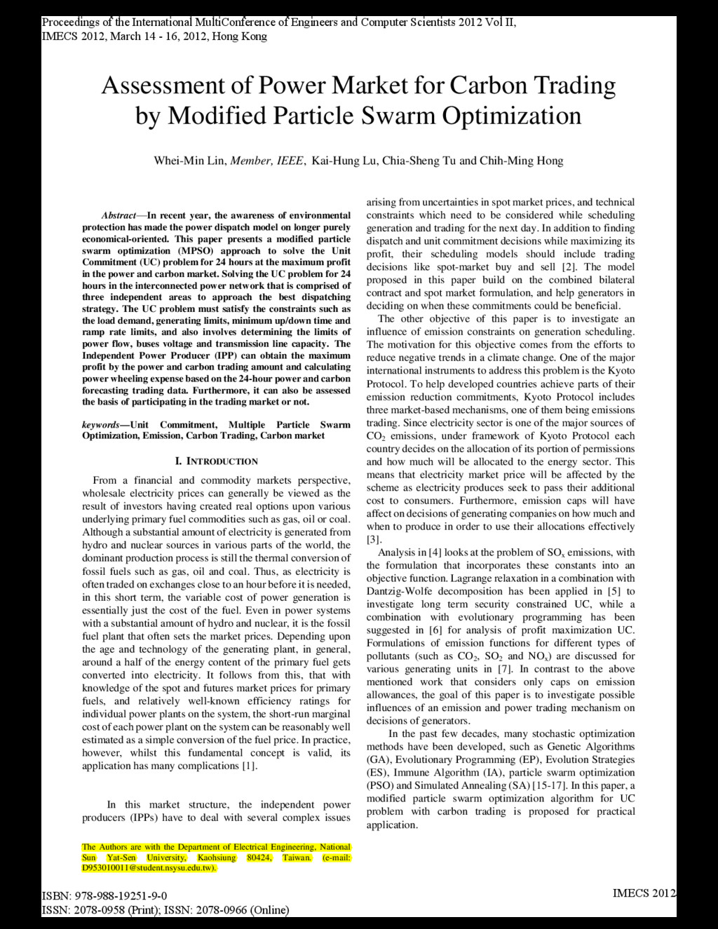
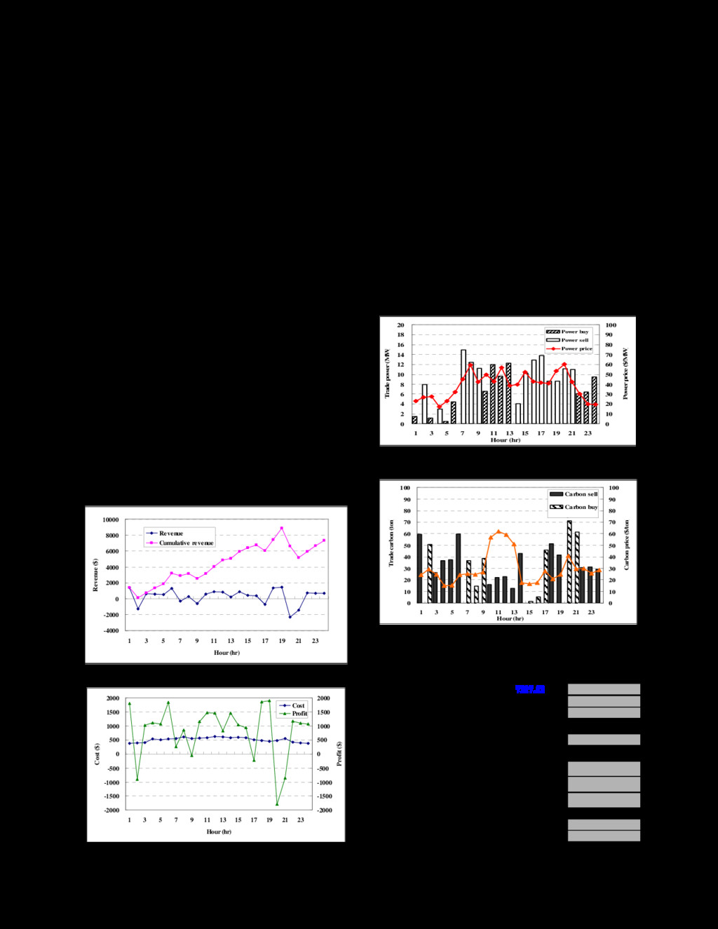
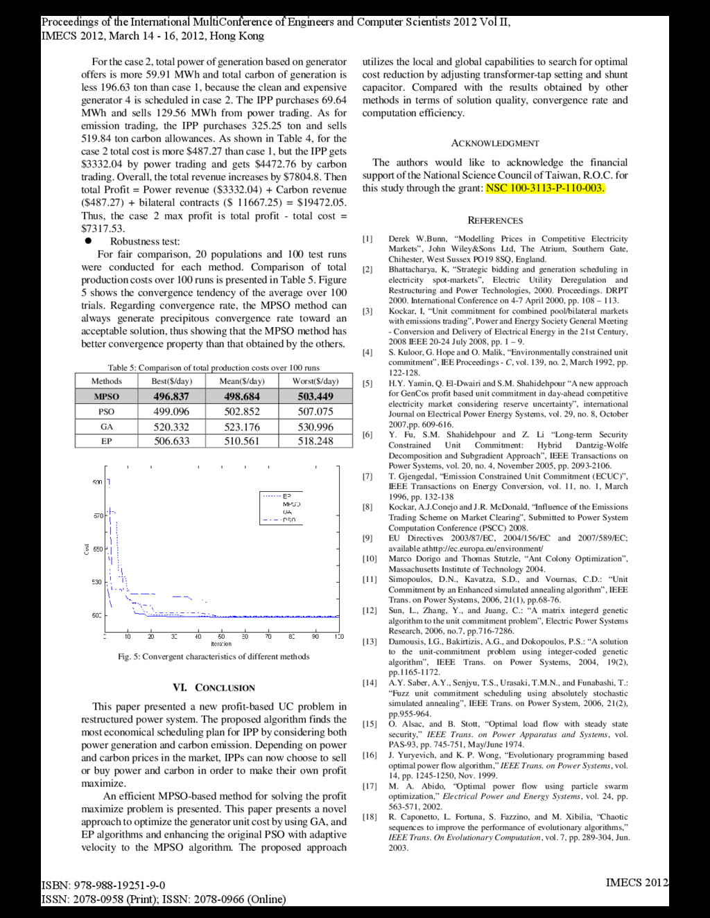
5. For the case 2, total power of generation based on generator offers is more 59.91 MWh and total carbon of generation is less 196.63 ton than case 1, because the clean and expensive generator 4 is scheduled in case 2. The IPP purchases 69.64 MWh and sells 129.56 MWh from power trading. As for emission trading, the IPP purchases 325.25 ton and sells 519.84 ton carbon allowances. As shown in Table 4, for the case 2 total cost is more $487.27 than case 1, but the IPP gets $3332.04 by power trading and gets $4472.76 by carbon trading. Overall, the total revenue increases by $7804.8. Then total Profit = Power revenue ($3332.04) + Carbon revenue ($487.27) + bilateral contracts ($ 11667.25) = $19472.05. Thus, the case 2 max profit is total profit - total cost = $7317.53. Robustness test: For fair comparison, 20 populations and 100 test runs were conducted for each method. Comparison of total production costs over 100 runs is presented in Table 5. Figure 5 shows the convergence tendency of the average over 100 trials. Regarding convergence rate, the MPSO method can always generate precipitous convergence rate toward an acceptable solution, thus showing that the MPSO method has better convergence property than that obtained by the others. Table 5: Comparison of total production costs over 100 runs Methods Best($/day) Mean($/day) Worst($/day) MPSO 496.837 498.684 503.449 PSO 499.096 502.852 507.075 GA 520.332 523.176 530.996 EP 506.633 510.561 518.248 Fig. 5: Convergent characteristics of different methods VI. CONCLUSION This paper presented a new profit-based UC problem in restructured power system. The proposed algorithm finds the most economical scheduling plan for IPP by considering both power generation and carbon emission. Depending on power and carbon prices in the market, IPPs can now choose to sell or buy power and carbon in order to make their own profit maximize. An efficient MPSO-based method for solving the profit maximize problem is presented. This paper presents a novel approach to optimize the generator unit cost by using GA, and EP algorithms and enhancing the original PSO with adaptive velocity to the MPSO algorithm. The proposed approach utilizes the local and global capabilities to search for optimal cost reduction by adjusting transformer-tap setting and shunt capacitor. Compared with the results obtained by other methods in terms of solution quality, convergence rate and computation efficiency. ACKNOWLEDGMENT The authors would like to acknowledge the financial support of the National Science Council of Taiwan, R.O.C. for this study through the grant: NSC 100-3113-P-110-003. REFERENCES [1] Derek W.Bunn, “Modelling Prices in Competitive Electricity Markets”, John Wiley&Sons Ltd, The Atrium, Southern Gate, Chihester, West Sussex PO19 8SQ, England. [2] Bhattacharya, K, “Strategic bidding and generation scheduling in electricity spot-markets”, Electric Utility Deregulation and Restructuring and Power Technologies, 2000. Proceedings. DRPT 2000. International Conference on 4-7 April 2000, pp. 108 – 113. [3] Kockar, I, “Unit commitment for combined pool/bilateral markets with emissions trading”, Power and Energy Society General Meeting - Conversion and Delivery of Electrical Energy in the 21st Century, 2008 IEEE 20-24 July 2008, pp. 1 – 9. [4] S. Kuloor, G. Hope and O. Malik, “Environmentally constrained unit commitment”, IEE Proceedings - C, vol. 139, no. 2, March 1992, pp. 122-128. [5] H.Y. Yamin, Q. El-Dwairi and S.M. Shahidehpour “A new approach for GenCos profit based unit commitment in day-ahead competitive electricity market considering reserve uncertainty”, international Journal on Electrical Power Energy Systems, vol. 29, no. 8, October 2007,pp. 609-616. [6] Y. Fu, S.M. Shahidehpour and Z. Li “Long-term Security Constrained Unit Commitment: Hybrid Dantzig-Wolfe Decomposition and Subgradient Approach”, IEEE Transactions on Power Systems, vol. 20, no. 4, November 2005, pp. 2093-2106. [7] T. Gjengedal, “Emission Constrained Unit Commitment (ECUC)”, IEEE Transactions on Energy Conversion, vol. 11, no. 1, March 1996, pp. 132-138 [8] Kockar, A.J.Conejo and J.R. McDonald, “Influence of the Emissions Trading Scheme on Market Clearing”, Submitted to Power System Computation Conference (PSCC) 2008. [9] EU Directives 2003/87/EC, 2004/156/EC and 2007/589/EC; available athttp://ec.europa.eu/environment/ [10] Marco Dorigo and Thomas Stutzle, “Ant Colony Optimization”, Massachusetts Institute of Technology 2004. [11] Simopoulos, D.N., Kavatza, S.D., and Vournas, C.D.: “Unit Commitment by an Enhanced simulated annealing algorithm”, IEEE Trans. on Power Systems, 2006, 21(1), pp.68-76. [12] Sun, L., Zhang, Y., and Juang, C.: “A matrix integerd genetic algorithm to the unit commitment problem”, Electric Power Systems Research, 2006, no.7, pp.716-7286. [13] Damousis, I.G., Bakirtizis, A.G., and Dokopoulos, P.S.: “A solution to the unit-commitment problem using integer-coded genetic algorithm”, IEEE Trans. on Power Systems, 2004, 19(2), pp.1165-1172. [14] A.Y. Saber, A.Y., Senjyu, T.S., Urasaki, T.M.N., and Funabashi, T.: “Fuzz unit commitment scheduling using absolutely stochastic simulated annealing”, IEEE Trans. on Power System, 2006, 21(2), pp.955-964. [15] O. Alsac, and B. Stott, “Optimal load flow with steady state security,” IEEE Trans. on Power Apparatus and Systems, vol. PAS-93, pp. 745-751, May/June 1974. [16] J. Yuryevich, and K. P. Wong, “Evolutionary programming based optimal power flow algorithm,” IEEE Trans. on Power Systems, vol. 14, pp. 1245-1250, Nov. 1999. [17] M. A. Abido, “Optimal power flow using particle swarm optimization,” Electrical Power and Energy Systems, vol. 24, pp. 563-571, 2002. [18] R. Caponetto, L. Fortuna, S. Fazzino, and M. Xibilia, “Chaotic sequences to improve the performance of evolutionary algorithms,” IEEE Trans. On Evolutionary Computation, vol. 7, pp. 289-304, Jun. 2003. Proceedings of the International MultiConference of Engineers and Computer Scientists 2012 Vol II, IMECS 2012, March 14 - 16, 2012, Hong Kong ISBN: 978-988-19251-9-0 ISSN: 2078-0958 (Print); ISSN: 2078-0966 (Online) IMECS 2012