Geometric calculations on probability manifolds from reciprocal relations in Master equations

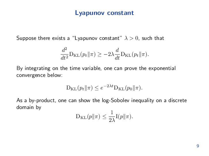
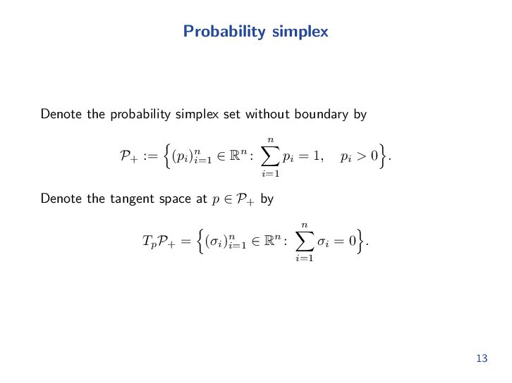
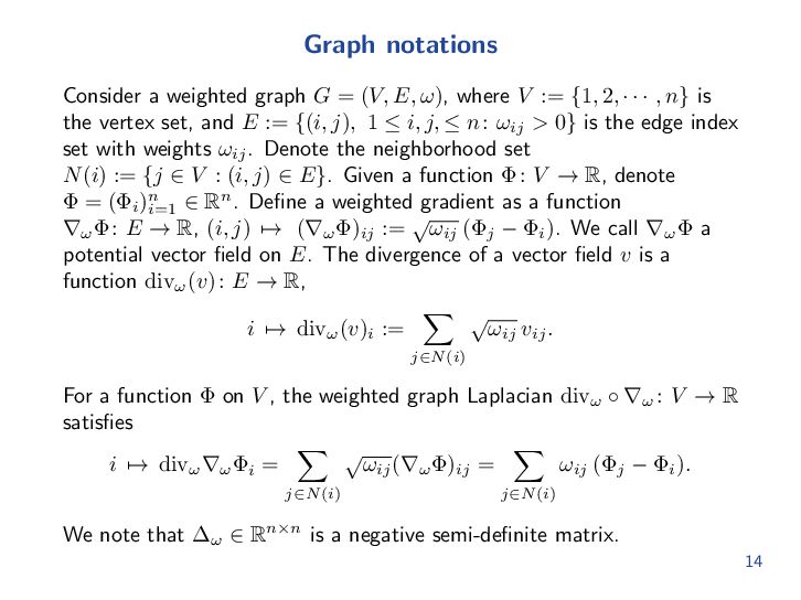
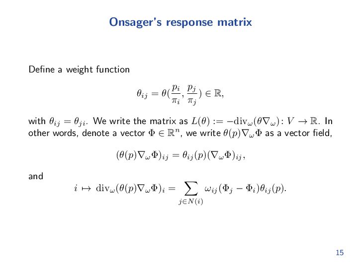
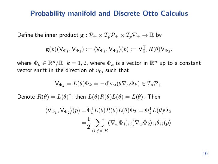
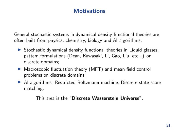
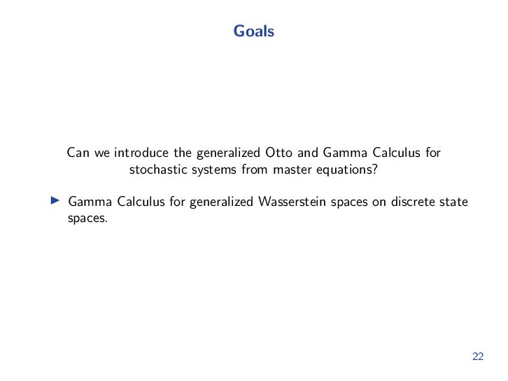
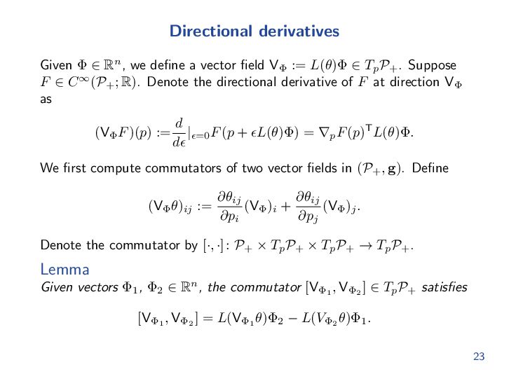
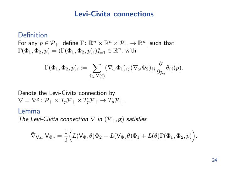
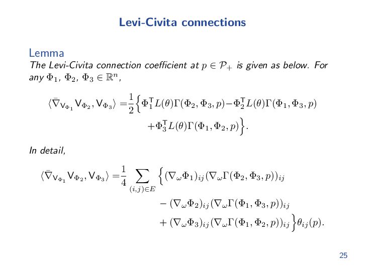
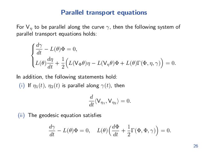
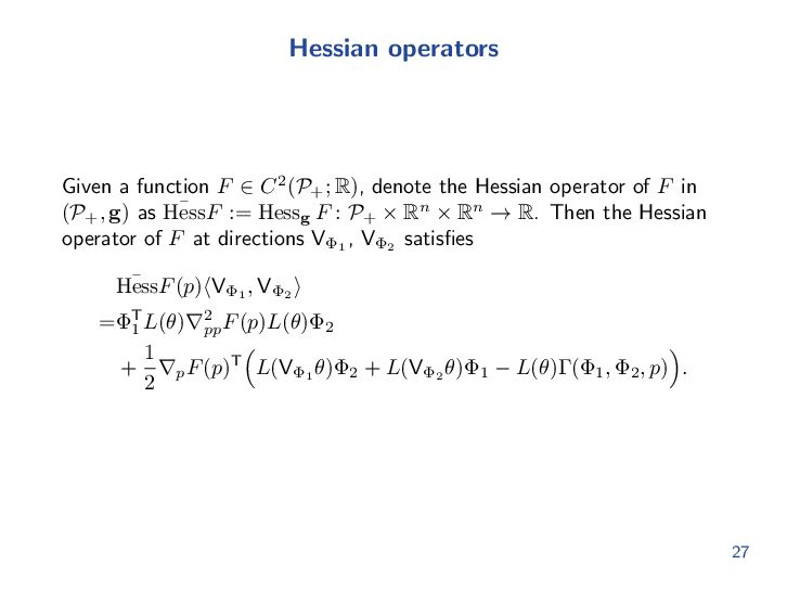
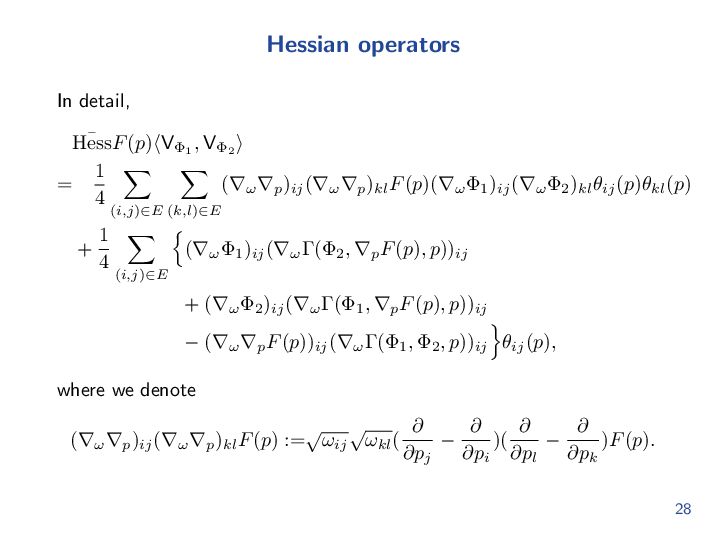
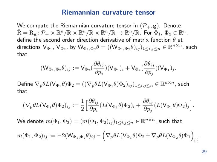
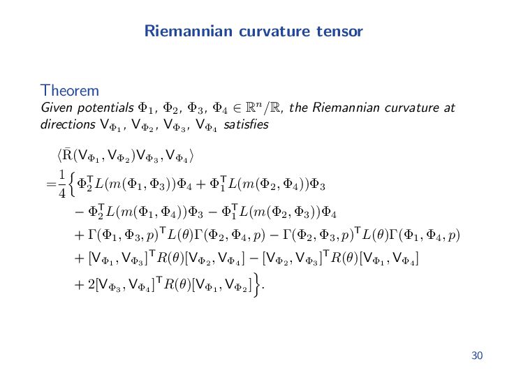
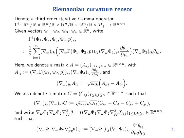
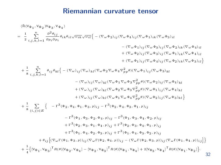
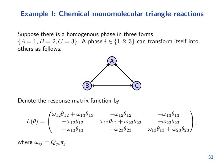
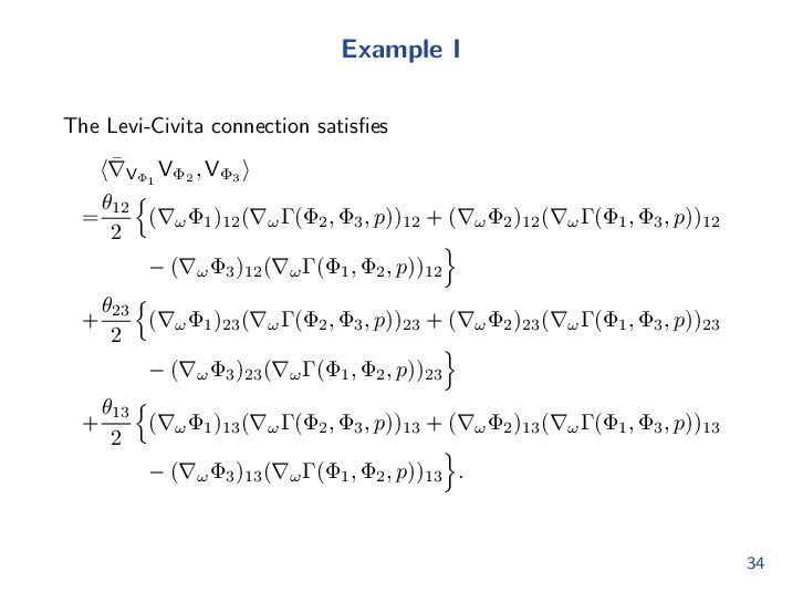
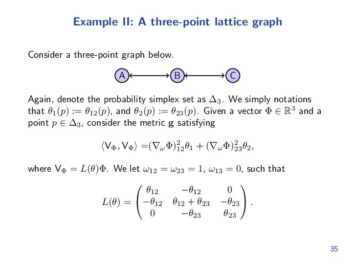
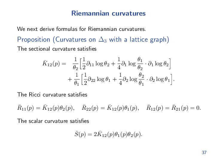
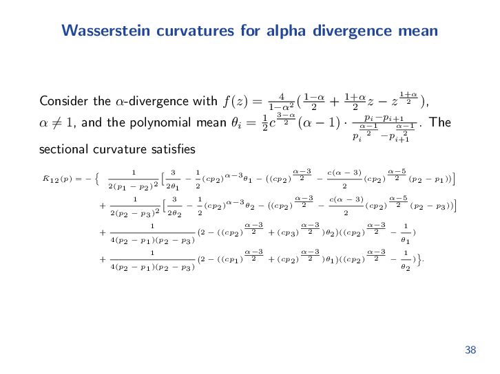
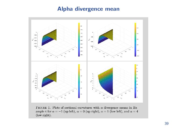
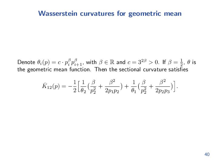
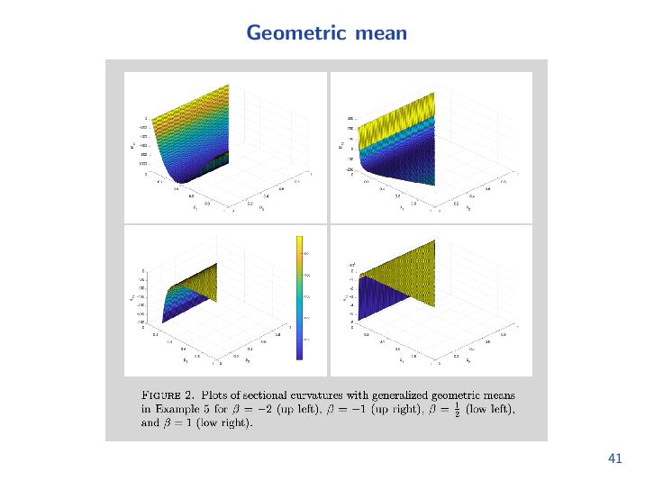
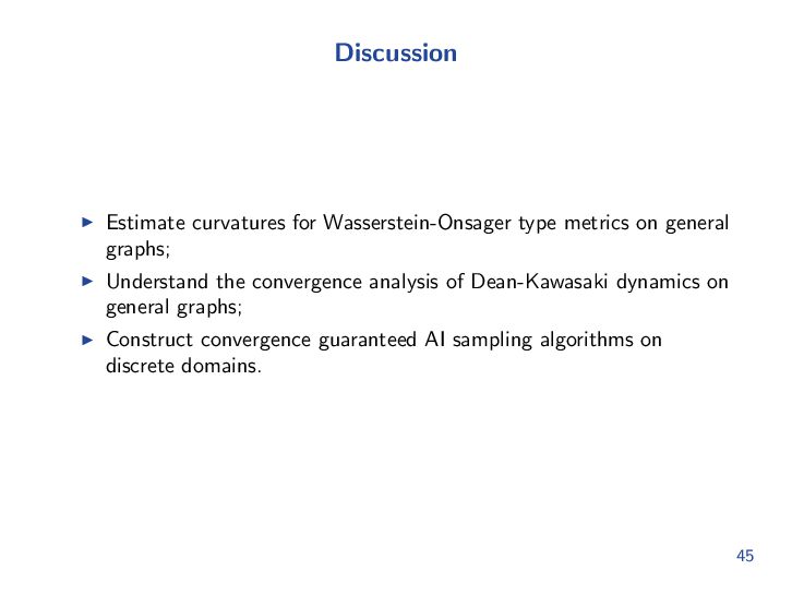
Onsager reciprocal relations model physical irreversible processes from complex systems. Recently, it has been shown that Onsager principles for master equations on finite states introduce a class of Riemannian metrics on the probability simplex, leading to probability manifolds or finite-state Wasserstein--2 spaces. In this paper, we study geometric calculations on probability manifolds, deriving the Levi-Civita connection, gradient, Hessian operators of energies, parallel transport, and calculating both the Riemannian and sectional curvatures. We present two examples of geometric quantities in probability manifolds. One example is the Levi-Civita connection from the chemical monomolecular triangle reaction. The other example is the sectional, Ricci, and scalar curvatures in Wasserstein space on a three-point lattice graph.

Transcript

1. Geometric calculations on probability manifolds from reciprocal relations in Master equations Wuchen Li University of South Carolina Spring Eastern Sectional Meeting at Boston College, MA, 2026. Supported from AFOSR YIP award, NSF RTG and FRG awards, and McCausland Fellowship award at University of South Carolina. 1
2. AI inference, Sampling, and Gamma calculus 2
3. Sampling problems Main problem Denote Ω = {1, 2, · · · , n}. Given a function V : Ω → R, the problem is to sample from πi = 1 Z e−Vi , where i ∈ Ω is a discrete sampling (state) space, π is a density function, and Z is a normalization constant. 3
4. Markov process Consider a discrete state 1, 2, · · · , n . Denote a probability distribution p(t) = (pi (t))n i=1 ∈ Rn + over states i = 1, 2, · · · , n, that characterizes the discrete state system in a time domain t ≥ 0, with 0 ≤ pi (t) ≤ 1, n i=1 pi (t) = 1. The master equation of the system 1, 2, · · · , n refers to the dynamical evolution of a probability function: dpi (t) dt = n j=1 Qji pj (t) − Qij pi (t) , where there is an initial value probability function p(0), and the nonnegative quantity Qji ≥ 0, 1 ≤ i ̸= j ≤ n, is the constant transition probability per time from state j to state i. 4
5. Detailed balance condition Definition Suppose that there exists a vector π = (πi )n i=1 ∈ Rn, with πi > 0 and n i=1 πi = 1, such that Qij πi = Qji πj , for i, j ∈ {1, 2, · · · , n}. From now on, we denote the symmetric weight function ω = (ωij )1≤i,j≤n ∈ Rn×n, such that ωij = ωji := Qji πj . 5
6. Example: Metropolis-Hastings algorithm Given a step size ∆t > 0, the discrete-time update of the master equation satisfies p(k+1) = p(k)P, P = In + Q∆t ∈ Rn×n, where In is the identity matrix. Given a user-specified conditional density qij = P(Y = j | X = i), also known as the candidate kernel, MH designs: Aij := A(X = i, Y = j) =      min πj qji πi qij , 1 , πi qij > 0; 1, πi qij = 0. Here the transition probability in Metropolis-Hastings algorithm satisfies QMH ij := qij Aij = min πj πi qji , qij . 6
7. Transport, Entropy and Information, Geometry 7
8. Lyapunov methods To study the dynamical behavior of pt , we apply a global Lyapunov functional: DKL (p∥π) = n i=1 pi log pi πi . Along the master equation, the first order dissipation satisfies d dt DKL (ρt ∥π) = − 1 2 n i,j=1 Qji πj (log pj πj − log pi πi )( pj πj − pi πi ) := − I. In literature, DKL is named the Kullback–Leibler divergence (relative entropy, also free energy in statistical physics community) and I is called the relative Fisher information functional. 8
9. Lyapunov constant Suppose there exists a “Lyapunov constant” λ > 0, such that d2 dt2 DKL (pt ∥π) ≥ −2λ d dt DKL (pt ∥π). By integrating on the time variable, one can prove the exponential convergence below: DKL (pt ∥π) ≤ e−2λtDKL (p0 ∥π). As a by-product, one can show the log-Sobolev inequality on a discrete domain by DKL (p∥π) ≤ 1 2λ I(p∥π). 9
10. Literature There are several mathematical, physical and information theoretical interests around above equalities. ▶ Iterative Gamma calculus (Bakry, Emery, et.al.); Geometric calculations in Density manifolds (Lafferty, Lott); ▶ Entropy dissipation and Hypocoercivity (Arnold, Carlen, Carrilo, Villani, Mohout, Jungel, Markowich, Toscani, et.al.); ▶ Optimal transport, displacement convexity and Hessian operators in density space. (McCann, Ambrosio, Villani, Otto, Gangbo, Mielke, Maas, Liero, et.al.); ▶ Wasserstein diffusion (Dean, Kawasaki, Renesse, Strum, et.al.); ▶ Discrete domain (Chow et al., Maas, and Mielke); Ricci curvatures and displacement convexities on Markov chains (Erbar, Maas, Mielke, Fathi, Li-Lu, et.al.); ▶ Wasserstein and Information geometry with applications in statistical physics (Ito, Kobayashi, et.al). 10
11. Optimal transport distances The optimal transport has a variational formulation (Benamou-Brenier 2000): D(ρ0, ρ1)2 := inf v 1 0 EXt∼ρt ∥v(t, Xt )∥2 dt, where E is the expectation operator and the infimum runs over all vector fields vt , such that ˙ Xt = v(t, Xt ), X0 ∼ ρ0, X1 ∼ ρ1. Under this metric, the probability set has a metric structure1. 1John D. Lafferty: the density manifold and configuration space quantization, 1988. 11
12. Otto Calculus on continuous states Informally speaking, the optimal transport metric refers to the following bilinear form: ⟨ ˙ ρ1 , G(ρ) ˙ ρ2 ⟩ = ( ˙ ρ1 , (−∇ · (ρ∇))−1 ˙ ρ2 )dx. In other words, denote ˙ ρi = −∇ · (ρ∇ϕi ), i = 1, 2, then ⟨ϕ1 , G(ρ)−1ϕ2 ⟩ = (∇ϕ1 , ∇ϕ2 )ρdx, where ρ ∈ P(Ω), ˙ ρi is the tangent vector in P(Ω), i.e. ˙ ρi dx = 0, and ϕi ∈ C∞(Ω) are cotangent vectors in P(Ω) at the point ρ. 12
13. Probability simplex Denote the probability simplex set without boundary by P+ := (pi )n i=1 ∈ Rn : n i=1 pi = 1, pi > 0 . Denote the tangent space at p ∈ P+ by Tp P+ = (σi )n i=1 ∈ Rn : n i=1 σi = 0 . 13
14. Graph notations Consider a weighted graph G = (V, E, ω), where V := {1, 2, · · · , n} is the vertex set, and E := {(i, j), 1 ≤ i, j, ≤ n: ωij > 0} is the edge index set with weights ωij . Denote the neighborhood set N(i) := {j ∈ V : (i, j) ∈ E}. Given a function Φ: V → R, denote Φ = (Φi )n i=1 ∈ Rn. Define a weighted gradient as a function ∇ω Φ: E → R, (i, j) → (∇ω Φ)ij := √ ωij (Φj − Φi ). We call ∇ω Φ a potential vector field on E. The divergence of a vector field v is a function divω (v): E → R, i → divω (v)i := j∈N(i) √ ωij vij . For a function Φ on V , the weighted graph Laplacian divω ◦ ∇ω : V → R satisfies i → divω ∇ω Φi = j∈N(i) √ ωij (∇ω Φ)ij = j∈N(i) ωij (Φj − Φi ). We note that ∆ω ∈ Rn×n is a negative semi-definite matrix. 14
15. Onsager’s response matrix Define a weight function θij = θ( pi πi , pj πj ) ∈ R, with θij = θji . We write the matrix as L(θ) := −divω (θ∇ω ): V → R. In other words, denote a vector Φ ∈ Rn, we write θ(p)∇ω Φ as a vector field, (θ(p)∇ω Φ)ij = θij (p)(∇ω Φ)ij , and i → divω (θ(p)∇ω Φ)i = j∈N(i) ωij (Φj − Φi )θij (p). 15
16. Probability manifold and Discrete Otto Calculus Define the inner product g : P+ × Tp P+ × Tp P+ → R by g(p)(VΦ1 , VΦ2 ) := ⟨VΦ1 , VΦ2 ⟩(p) := VT Φ1 R(θ)VΦ2 , where Φk ∈ Rn/R, k = 1, 2, where Φk is a vector in Rn up to a constant vector shrift in the direction of u0 , such that VΦk = L(θ)Φk = −divω (θ∇ω Φk ) ∈ Tp P+ . Denote R(θ) = L(θ)†, then L(θ)R(θ)L(θ) = L(θ). Then ⟨VΦ1 , VΦ2 ⟩(p) =ΦT 1 L(θ)R(θ)L(θ)Φ2 = ΦT 1 L(θ)Φ2 = 1 2 (i,j)∈E (∇ω Φ1 )ij (∇ω Φ2 )ij θij (p). 16
17. Gradient operators Denote an energy function F ∈ C∞(P+ ; R). The gradient operator of function F in (P+ , g) satisfies ¯ gradF(p) = L(θ)∇p F(p) = −divω (θ∇ω ∇p F(p)). In particular, if F(p) = Df (p∥π) = n i=1 f(pi πi )πi , and θij = pi πi − pj πj f′(pj πj ) − f′(pi πi ) , then the negative gradient direction of f-divergence satisfies the R.H.S. of master equation: − ¯ gradDf (p∥π) = − L(θ)∇p Df (p∥π) =divω (θ∇ω ∇p Df (p∥π)) = n j=1 Qji pj − Qij pi n i=1 . 17
18. First order calculus Denote f(z) = z log z − z. One can study the first order entropy dissipation as follows. d dt DKL (ρt ∥π) = − (∇p DKL (ρt ∥π))TL(θ)∇p DKL (ρt ∥π) = − 1 2 n i,j=1 ωij (log pj πj − log pi πi )2θij ≤ 0. 18
19. Master equations as Onsager gradient flows Proposition (Onsager reciprocal relations) Master equation can be rewritten as dp(t) dt = −L(θ(p(t)))∇p Df (p(t)∥π), where ∇p Df (p∥π) is the generalized force and L(θ) is the Onsager’s response matrix. In addition, along with the solution of the master equation (4), the free energy Df (p(t)∥π) decays in the time variable. d dt Df (p(t)∥π) = −∇p Df (p(t)∥π)TL(θ(p(t)))∇p Df (p(t)∥π) ≤ 0. 19
20. Distances Proposition (Arc length function) For a curve γ ∈ C1([0, T]; P+ ), where T > 0, the arc length Leng (γ) of curve γ is defined as Leng (γ) := T 0 ˙ γ(t)TR(θ(γ(t)))˙ γ(t) 1 2 dt. Definition (Minimal arc length problems and Distances) Given two points p0, p1 ∈ P+ . The minimal arc length problem satisfies the following optimization problem: Dist(p0, p1) := inf γ Leng (γ): γ(0) = p0, γ(1) = p1 , where the minimization is taken over all continuous differentiable curves in the probability simplex set, γ(t) ∈ C1([0, 1]; P+ ), t ∈ [0, 1], connecting boundary points γ(0) = p0, γ(1) = p1. 20
21. Motivations General stochastic systems in dynamical density functional theories are often built from physics, chemistry, biology and AI algorithms. ▶ Stochastic dynamical density functional theories in Liquid glasses, pattern formulations (Dean, Kawasaki, Li, Gao, Liu, etc...) on discrete domains; ▶ Macroscopic fluctuation theory (MFT) and mean field control problems on discrete domains; ▶ AI algorithms: Restricted Boltzmann machine; Discrete state score matching. This area is the “Discrete Wasserstein Universe”. 21
22. Goals Can we introduce the generalized Otto and Gamma Calculus for stochastic systems from master equations? ▶ Gamma Calculus for generalized Wasserstein spaces on discrete state spaces. 22
23. Directional derivatives Given Φ ∈ Rn, we define a vector field VΦ := L(θ)Φ ∈ Tp P+ . Suppose F ∈ C∞(P+ ; R). Denote the directional derivative of F at direction VΦ as (VΦ F)(p) := d dϵ |ϵ=0 F(p + ϵL(θ)Φ) = ∇p F(p)TL(θ)Φ. We first compute commutators of two vector fields in (P+ , g). Define (VΦ θ)ij := ∂θij ∂pi (VΦ )i + ∂θij ∂pj (VΦ )j . Denote the commutator by [·, ·]: P+ × Tp P+ × Tp P+ → Tp P+ . Lemma Given vectors Φ1 , Φ2 ∈ Rn, the commutator [VΦ1 , VΦ2 ] ∈ Tp P+ satisfies [VΦ1 , VΦ2 ] = L(VΦ1 θ)Φ2 − L(VΦ2 θ)Φ1 . 23
24. Levi-Civita connections Definition For any p ∈ P+ , define Γ: Rn × Rn × P+ → Rn, such that Γ(Φ1 , Φ2 , p) = (Γ(Φ1 , Φ2 , p)i )n i=1 ∈ Rn, with Γ(Φ1 , Φ2 , p)i := j∈N(i) (∇ω Φ1 )ij (∇ω Φ2 )ij ∂ ∂pi θij (p). Denote the Levi-Civita connection by ¯ ∇ = ∇g : P+ × Tp P+ × Tp P+ → Tp P+ . Lemma The Levi-Civita connection ¯ ∇ in (P+ , g) satisfies ¯ ∇VΦ1 VΦ2 = 1 2 L(VΦ1 θ)Φ2 − L(VΦ2 θ)Φ1 + L(θ)Γ(Φ1 , Φ2 , p) . 24
25. Levi-Civita connections Lemma The Levi-Civita connection coefficient at p ∈ P+ is given as below. For any Φ1 , Φ2 , Φ3 ∈ Rn, ⟨ ¯ ∇VΦ1 VΦ2 , VΦ3 ⟩ = 1 2 ΦT 1 L(θ)Γ(Φ2 , Φ3 , p)−ΦT 2 L(θ)Γ(Φ1 , Φ3 , p) +ΦT 3 L(θ)Γ(Φ1 , Φ2 , p) . In detail, ⟨ ¯ ∇VΦ1 VΦ2 , VΦ3 ⟩ = 1 4 (i,j)∈E (∇ω Φ1 )ij (∇ω Γ(Φ2 , Φ3 , p))ij − (∇ω Φ2 )ij (∇ω Γ(Φ1 , Φ3 , p))ij + (∇ω Φ3 )ij (∇ω Γ(Φ1 , Φ2 , p))ij θij (p). 25
26. Parallel transport equations For Vη to be parallel along the curve γ, then the following system of parallel transport equations holds:      dγ dt − L(θ)Φ = 0, L(θ) dη dt + 1 2 L(VΦ θ)η − L(Vη θ)Φ + L(θ)Γ(Φ, η, γ) = 0. In addition, the following statements hold: (i) If η1 (t), η2 (t) is parallel along γ(t), then d dt ⟨Vη1 , Vη2 ⟩ = 0. (ii) The geodesic equation satisfies dγ dt − L(θ)Φ = 0, L(θ) dΦ dt + 1 2 Γ(Φ, Φ, γ) = 0. 26
27. Hessian operators Given a function F ∈ C2(P+ ; R), denote the Hessian operator of F in (P+ , g) as ¯ HessF := Hessg F : P+ × Rn × Rn → R. Then the Hessian operator of F at directions VΦ1 , VΦ2 satisfies ¯ HessF(p)⟨VΦ1 , VΦ2 ⟩ =ΦT 1 L(θ)∇2 pp F(p)L(θ)Φ2 + 1 2 ∇p F(p)T L(VΦ1 θ)Φ2 + L(VΦ2 θ)Φ1 − L(θ)Γ(Φ1 , Φ2 , p) . 27
28. Hessian operators In detail, ¯ HessF(p)⟨VΦ1 , VΦ2 ⟩ = 1 4 (i,j)∈E (k,l)∈E (∇ω ∇p )ij (∇ω ∇p )kl F(p)(∇ω Φ1 )ij (∇ω Φ2 )kl θij (p)θkl (p) + 1 4 (i,j)∈E (∇ω Φ1 )ij (∇ω Γ(Φ2 , ∇p F(p), p))ij + (∇ω Φ2 )ij (∇ω Γ(Φ1 , ∇p F(p), p))ij − (∇ω ∇p F(p))ij (∇ω Γ(Φ1 , Φ2 , p))ij θij (p), where we denote (∇ω ∇p )ij (∇ω ∇p )kl F(p) := √ ωij √ ωkl ( ∂ ∂pj − ∂ ∂pi )( ∂ ∂pl − ∂ ∂pk )F(p). 28
29. Riemannian curvature tensor We compute the Riemannian curvature tensor in (P+ , g). Denote ¯ R = Rg : P+ × Rn/R × Rn/R × Rn/R → Rn/R. For Φ1 , Φ2 ∈ Rn, define the second order direction derivative of matrix function θ at directions VΦ1 , VΦ2 , by WΦ1,Φ2 θ = ((WΦ1,Φ2 θ)ij )1≤i,j≤n ∈ Rn×n, such that (WΦ1,Φ2 θ)ij := VΦ2 ( ∂θij ∂pi )(VΦ1 )i + VΦ2 ( ∂θij ∂pj )(VΦ1 )j . Define ∇p θL(VΦ1 θ)Φ2 = ((∇p θL(VΦ1 θ)Φ2 )ij )1≤i,j≤n ∈ Rn×n, such that (∇p θL(VΦ1 θ)Φ2 )ij := 1 2 ∂θij ∂pi (L(VΦ1 θ)Φ2 )i + ∂θij ∂pj (L(VΦ1 θ)Φ2 )j . We denote m(Φ1 , Φ2 ) = (m(Φ1 , Φ2 )ij )1≤i,j≤n ∈ Rn×n, such that m(Φ1 , Φ2 )ij := −2(WΦ1,Φ2 θ)ij − ∇p θL(VΦ1 θ)Φ2 + ∇p θL(VΦ2 θ)Φ1 ij . 29
30. Riemannian curvature tensor Theorem Given potentials Φ1 , Φ2 , Φ3 , Φ4 ∈ Rn/R, the Riemannian curvature at directions VΦ1 , VΦ2 , VΦ3 , VΦ4 satisfies ⟨¯ R(VΦ1 , VΦ2 )VΦ3 , VΦ4 ⟩ = 1 4 ΦT 2 L(m(Φ1 , Φ3 ))Φ4 + ΦT 1 L(m(Φ2 , Φ4 ))Φ3 − ΦT 2 L(m(Φ1 , Φ4 ))Φ3 − ΦT 1 L(m(Φ2 , Φ3 ))Φ4 + Γ(Φ1 , Φ3 , p)TL(θ)Γ(Φ2 , Φ4 , p) − Γ(Φ2 , Φ3 , p)TL(θ)Γ(Φ1 , Φ4 , p) + [VΦ1 , VΦ3 ]TR(θ)[VΦ2 , VΦ4 ] − [VΦ2 , VΦ3 ]TR(θ)[VΦ1 , VΦ4 ] + 2[VΦ3 , VΦ4 ]TR(θ)[VΦ1 , VΦ2 ] . 30
31. Riemannian curvature tensor Denote a third order iterative Gamma operator Γ3 : Rn/R × Rn/R × Rn/R × Rn/R × P+ → Rn×n. Given vectors Φ1 , Φ2 , Φ3 , Φ4 ∈ Rn, write Γ3(Φ1 , Φ2 , Φ3 , Φ4 , p)ij := 1 2 n k=1 (∇ω )ik (∇ω Γ(Φ1 , Φ2 , p))ij (∇ω Φ4 )ij ∂θij ∂pi (∇ω Φ3 )ik θik . Here, we denote a matrix A = (Aij )i≤i,j≤n ∈ Rn×n, with Aij := (∇ω Γ(Φ1 , Φ2 , p))ij (∇ω Φ4 )ij ∂θij ∂pi , and (∇ω )ik Aij := √ ωik Akj − Aij . We also denote a matrix C = (Cij )1≤i,j≤n ∈ Rn×n, such that (∇ω )ij (∇ω )kl C := √ ωij √ ωkl (Cik − Cil − Cjk + Cjl ), and write ∇ω Φ1 ∇ω Φ2 ∇2 pp θ = ((∇ω Φ1 ∇ω Φ2 ∇2 pp θ)ij )1≤i,j≤n ∈ Rn×n, such that (∇ω Φ1 ∇ω Φ2 ∇2 pp θ)ij := (∇ω Φ1 )ij (∇ω Φ2 )ij ∂2θij ∂pi ∂pj . 31
32. Riemannian curvature tensor ⟨¯ R(VΦ1 , VΦ2 )VΦ3 , VΦ4 ⟩ = 1 2 n i,j,k,l=1 ∂2θij ∂pi∂pi θikθil √ ωik √ ωil − (∇ωΦ2)ij (∇ωΦ4)ij (∇ωΦ1)ik(∇ωΦ3)il − (∇ωΦ1)ij (∇ωΦ3)ij (∇ωΦ2)ik(∇ωΦ4)il + (∇ωΦ2)ij (∇ωΦ3)ij (∇ωΦ1)ik(∇ωΦ4)il + (∇ωΦ1)ij (∇ωΦ4)ij (∇ωΦ2)ik(∇ωΦ3)il + 1 8 n i,j,k,l=1 θij θkl − (∇ω)ij (∇ω)kl(∇ωΦ2∇ωΦ4∇ 2 ppθ)(∇ωΦ1)ij (∇ωΦ3)kl − (∇ω)ij (∇ω)kl(∇ωΦ1∇ωΦ3∇ 2 ppθ)(∇ωΦ2)ij (∇ωΦ4)kl + (∇ω)ij (∇ω)kl(∇ωΦ2∇ωΦ3∇ 2 ppθ)(∇ωΦ1)ij (∇ωΦ4)kl + (∇ω)ij (∇ω)kl(∇ωΦ1∇ωΦ4∇ 2 ppθ)(∇ωΦ2)ij (∇ωΦ3)kl + 1 8 (i,j)∈E − Γ 3 (Φ2, Φ4, Φ1, Φ3, p)ij − Γ 3 (Φ2, Φ4, Φ3, Φ1, p)ij − Γ 3 (Φ1, Φ3, Φ2, Φ4, p)ij − Γ 3 (Φ1, Φ3, Φ4, Φ2, p)ij + Γ 3 (Φ2, Φ3, Φ1, Φ4, p)ij + Γ 3 (Φ2, Φ3, Φ4, Φ1, p)ij + Γ 3 (Φ1, Φ4, Φ2, Φ3, p)ij + Γ 3 (Φ1, Φ4, Φ3, Φ2, p)ij + θij (∇ωΓ(Φ1, Φ3, p))ij (∇ωΓ(Φ2, Φ4, p))ij − (∇ωΓ(Φ2, Φ3, p))ij (∇ωΓ(Φ1, Φ4, p))ij + 1 4 [VΦ1 , VΦ3 ] T R(θ)[VΦ2 , VΦ4 ] − [VΦ2 , VΦ3 ] T R(θ)[VΦ1 , VΦ4 ] + 2[VΦ3 , VΦ4 ] T R(θ)[VΦ1 , VΦ2 ] . 32
33. Example I: Chemical monomolecular triangle reactions Suppose there is a homogenous phase in three forms {A = 1, B = 2, C = 3}. A phase i ∈ {1, 2, 3} can transform itself into others as follows. A C B Denote the response matrix function by L(θ) =   ω12 θ12 + ω13 θ13 −ω12 θ12 −ω13 θ13 −ω12 θ12 ω12 θ12 + ω23 θ23 −ω23 θ23 −ω13 θ13 −ω23 θ23 ω13 θ13 + ω23 θ23   , where ωij = Qji πj . 33
34. Example I The Levi-Civita connection satisfies ⟨ ¯ ∇VΦ1 VΦ2 , VΦ3 ⟩ = θ12 2 (∇ω Φ1 )12 (∇ω Γ(Φ2 , Φ3 , p))12 + (∇ω Φ2 )12 (∇ω Γ(Φ1 , Φ3 , p))12 − (∇ω Φ3 )12 (∇ω Γ(Φ1 , Φ2 , p))12 + θ23 2 (∇ω Φ1 )23 (∇ω Γ(Φ2 , Φ3 , p))23 + (∇ω Φ2 )23 (∇ω Γ(Φ1 , Φ3 , p))23 − (∇ω Φ3 )23 (∇ω Γ(Φ1 , Φ2 , p))23 + θ13 2 (∇ω Φ1 )13 (∇ω Γ(Φ2 , Φ3 , p))13 + (∇ω Φ2 )13 (∇ω Γ(Φ1 , Φ3 , p))13 − (∇ω Φ3 )13 (∇ω Γ(Φ1 , Φ2 , p))13 . 34
35. Example II: A three-point lattice graph Consider a three-point graph below. A B C Again, denote the probability simplex set as ∆3 . We simply notations that θ1 (p) := θ12 (p), and θ2 (p) := θ23 (p). Given a vector Φ ∈ R3 and a point p ∈ ∆3 , consider the metric g satisfying ⟨VΦ , VΦ ⟩ =(∇ω Φ)2 12 θ1 + (∇ω Φ)2 23 θ2 , where VΦ = L(θ)Φ. We let ω12 = ω23 = 1, ω13 = 0, such that L(θ) =   θ12 −θ12 0 −θ12 θ12 + θ23 −θ23 0 −θ23 θ23   . 35
36. Cumulative distribution coordinates There is a particular coordinate for ∆3 , which simplifies geometric calculations. Denote the cumulative distribution function (CDF) on discrete states, such that x1 = p1 , x2 = p1 + p2 . Denote a set CDF = {(x1 , x2 ) ∈ [0, 1]2 : x1 ≤ x2 }. Thus, the metric g in coordinates (x1 , x2 ) is a diagonal matrix, such that g = (gij )1≤i,j≤2 ∈ R2×2, with g11 = 1 θ1 (x) , g22 = 1 θ2 (x) , g12 = g21 = 0. 36
37. Riemannian curvatures We next derive formulas for Riemannian curvatures. Proposition (Curvatures on ∆3 with a lattice graph) The sectional curvature satisfies ¯ K12 (p) = 1 θ2 1 2 ∂11 log θ2 + 1 4 ∂1 log θ1 θ2 · ∂1 log θ2 + 1 θ1 1 2 ∂22 log θ1 + 1 4 ∂2 log θ2 θ1 · ∂2 log θ1 . The Ricci curvature satisfies ¯ R11 (p) = ¯ K12 (p)θ2 (p), ¯ R22 (p) = ¯ K12 (p)θ1 (p), ¯ R12 (p) = ¯ R21 (p) = 0. The scalar curvature satisfies ¯ S(p) = 2 ¯ K12 (p)θ1 (p)θ2 (p). 37
38. Wasserstein curvatures for alpha divergence mean Consider the α-divergence with f(z) = 4 1−α2 (1−α 2 + 1+α 2 z − z 1+α 2 ), α ̸= 1, and the polynomial mean θi = 1 2 c3−α 2 (α − 1) · pi−pi+1 p α−1 2 i −p α−1 2 i+1 . The sectional curvature satisfies ¯ K12(p) = − 1 2(p1 − p2)2 3 2θ1 − 1 2 (cp2) α−3 θ1 − (cp2) α−3 2 − c(α − 3) 2 (cp2) α−5 2 (p2 − p1) + 1 2(p2 − p3)2 3 2θ2 − 1 2 (cp2) α−3 θ2 − (cp2) α−3 2 − c(α − 3) 2 (cp2) α−5 2 (p2 − p3) + 1 4(p2 − p1)(p2 − p3) 2 − ((cp2) α−3 2 + (cp3) α−3 2 )θ2 ((cp2) α−3 2 − 1 θ1 ) + 1 4(p2 − p1)(p2 − p3) 2 − ((cp1) α−3 2 + (cp2) α−3 2 )θ1 ((cp2) α−3 2 − 1 θ2 ) . 38
39. Alpha divergence mean 39
40. Wasserstein curvatures for geometric mean Denote θi (p) = c · pβ i pβ i+1 , with β ∈ R and c = 32β > 0. If β = 1 2 , θ is the geometric mean function. Then the sectional curvature satisfies ¯ K12 (p) = − 1 2 1 θ2 β p2 2 + β2 2p1 p2 + 1 θ1 β p2 2 + β2 2p2 p3 . 40
41. Geometric mean 41
42. Discussion ▶ Estimate curvatures for Wasserstein-Onsager type metrics on general graphs; ▶ Understand the convergence analysis of Dean-Kawasaki dynamics on general graphs; ▶ Construct convergence guaranteed AI sampling algorithms on discrete domains. 42