Geometric calculations on density manifolds from reciprocal relations in hydrodynamics

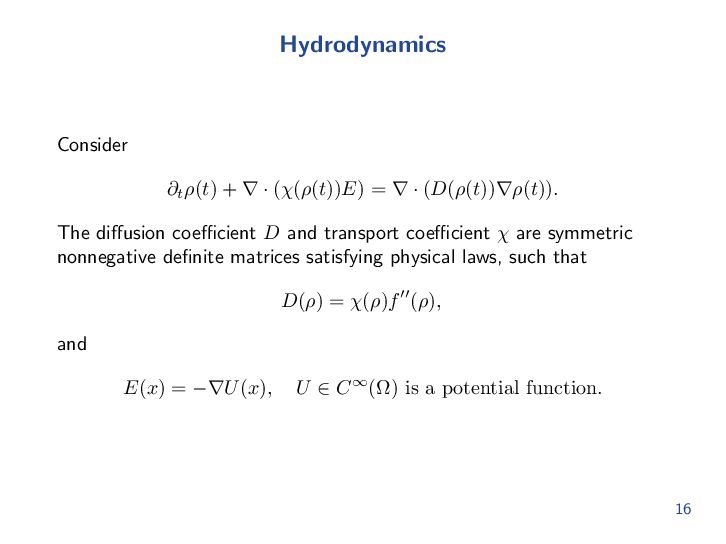
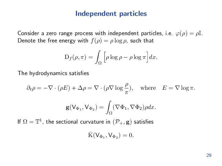
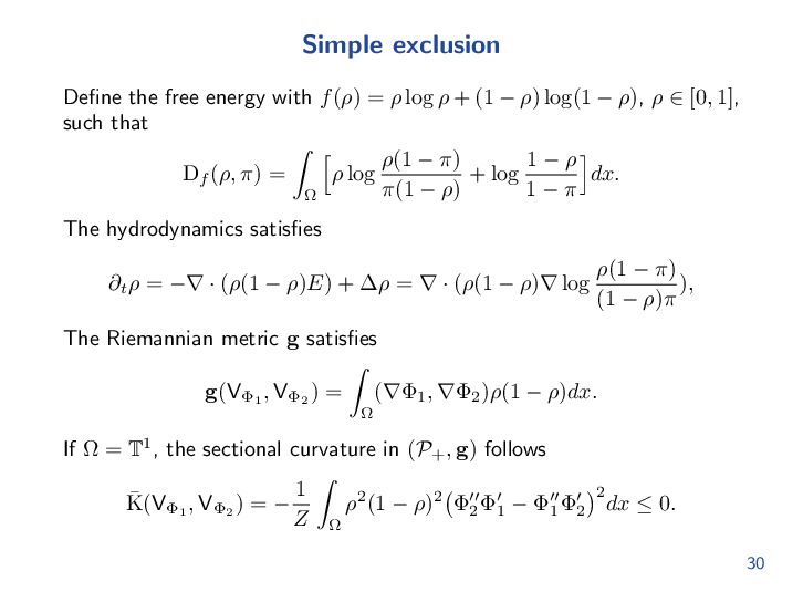
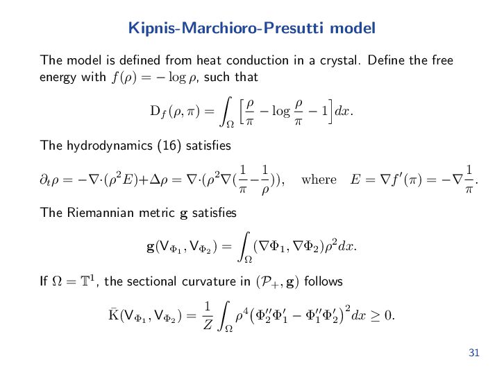
Hydrodynamics describes the evolution of macroscopic states in non–equilibrium thermodynamics. Following Onsager reciprocal relations, one can formulate a large class of hydrodynamic equations as gradient flows of free energies. In recent years, such Onsager gradient flows have been extensively investigated on optimal transport type metric spaces with nonlinear mobilities, known as hydrodynamical density manifolds. A typical example is the gradient–drift Fokker–Planck equation, which can be characterized as the gradient flow of the free energy in the Wasserstein-2 metric space. This paper studies geometric calculations on general hydrodynamical density manifolds. We first formulate the associated Levi–Civita connections, gradients, Hessians, and parallel transports, and then derive the corresponding Riemannian and sectional curvatures. Finally, we obtain closed-form formulas for sectional curvatures in one dimensional density manifolds, where the signs of the curvatures are determined by the convexity of the mobility functions. As illustrations, we present density manifolds and their sectional curvatures for several zero range models, including independent particle systems, simple exclusion processes, and Kipnis–Marchioro–Presutti models.

Transcript

1. Geometric calculations on density manifolds from reciprocal relations in hydrodynamics Wuchen Li University of South Carolina MPI MIS, Germany, July 15, 2025. Supported from AFOSR YIP award, NSF RTG and FRG awards, and McCausland Fellowship award at University of South Carolina. 1
2. AI modeling, inference and Sampling 2
3. Sampling problems Main problem Given a function V : Ω → R, the problem is to sample from π(x) = 1 Z e−V (x), where x ∈ Ω is a discrete or continuous sampling (state) space, π is a probability density function, and Z is a normalization constant. Difficulties ▶ Fast, efficient, accurate algorithms; ▶ High dimensional sampling: Ω ⊂ RN , N >> 3. E.g., Image distributions Ω = R64∗64; ▶ Function V = − log π − log Z, is often unknown or with intractable formulations. For simplicity of talk, we assume V or π is analytical known. 3
4. Stochastic differential equations Consider a stochastic differential equation (SDE) by ˙ Xt = b(Xt ) + √ 2a(Xt ) ˙ Bt , where (n, m) ∈ N, Xt ∈ Rn+m, b ∈ Rn+m is a drift vector function, a(Xt ) ∈ R(n+m)×n is a diffusion matrix function, and Bt ∈ Rn is a standard n dimensional Brownian motion. For a diffusion matrix a and drift vector field b, assume that it has an invariant measure of shape π, how can we analyze the convergence speed of stochastic dynamics towards its invariant distribution? This is crucial in designing AI type sampling algorithms. 4
5. Transport, Entropy and Information, Geometry 5
6. Example: Langevin dynamics We review a classical example. Consider an overdamped Langevin dynamics in Rn: ˙ Xt = −∇V (Xt ) + √ 2 ˙ Bt , where V is a given potential function. Let ρ(t, x) be the probability density function of Xt , which satisfies the following Fokker-Planck equation ∂t ρ(t, x) = L∗ρ(t, x) = ∇ · (ρ(t, x)∇V (x)) + ∆ρ(t, x). Here π(x) := 1 Z e−V (x), Z = e−V (y)dy < ∞, is the invariant distribution of the SDE. 6
7. Lyapunov methods To study the dynamical behavior of ρ, we apply a global Lyapunov functional: DKL (ρt ∥π) = ρt (x)log ρt (x) π(x) dx. Along the Fokker-Planck equation, the first order dissipation satisfies d dt DKL (ρt ∥π) = − ∥∇x log ρt (x) π(x) ∥2ρt dx. And the second order dissipation satisfies d2 dt2 DKL (ρt ∥π) = 2 ∥∇2 xx log ρt π ∥2 F −∇2 xx log π(∇x log ρt π , ∇x log ρt π ) ρt dx, where ∥ · ∥F is a matrix Frobenius norm. In literature, DKL is named the Kullback–Leibler divergence (relative entropy, also free energy in statistical physics community) and I = − d dt DKL is called the relative Fisher information functional. 7
8. Lyapunov constant Suppose there exists a “Lyapunov constant” λ > 0, such that −∇2 xx log π(x) ⪰ λI. Then d2 dt2 DKL (ρt ∥π) ≥ −2λ d dt DKL (ρt ∥π). By integrating on the time variable, one can prove the exponential convergence below: DKL (ρt ∥π) ≤ e−2λtDKL (ρ0 ∥π). 8
9. Literature There are several interesting mathematics and physics behind above equalities. ▶ Iterative Gamma calculus (Bakry, Emery, et.al.); ▶ Density manifolds (Lafferty, Lott); ▶ Entropy dissipation and Hypocoercivity (Arnold, Carlen, Carrilo, Villani, Mohout, Jungel, Markowich, Toscani, et.al.); ▶ Optimal transport, displacement convexity and Hessian operators in density space. (McCann, Ambrosio, Villani, Otto, Gangbo, Mielke, Maas, Liero, et.al.); ▶ Transport Lyapunov functional (Renesse, Strum et.al.). 9
10. Optimal transport distances The optimal transport has a variational formulation (Benamou-Brenier 2000): D(ρ0, ρ1)2 := inf v 1 0 EXt∼ρt ∥v(t, Xt )∥2 dt, where E is the expectation operator and the infimum runs over all vector fields vt , such that ˙ Xt = v(t, Xt ), X0 ∼ ρ0, X1 ∼ ρ1. Under this metric, the probability set has a metric structure1. 1John D. Lafferty: the density manifold and configuration space quantization, 1988. 10
11. Optimal transport metrics and Otto Calculuses Informally speaking, the optimal transport metric refers to the following bilinear form: ⟨ ˙ ρ1 , G(ρ) ˙ ρ2 ⟩ = ( ˙ ρ1 , (−∇ · (ρ∇))−1 ˙ ρ2 )dx. In other words, denote ˙ ρi = −∇ · (ρ∇ϕi ), i = 1, 2, then ⟨ϕ1 , G(ρ)−1ϕ2 ⟩ = (ϕ1 , −∇ · (ρ∇)ϕ2 )dx = (∇ϕ1 , ∇ϕ2 )ρdx, where ρ ∈ P(Ω), ˙ ρi is the tangent vector in P(Ω), i.e. ˙ ρi dx = 0, and ϕi ∈ C∞(Ω) are cotangent vectors in P(Ω) at the point ρ. 11
12. Optimal transport gradient operators The Wasserstein gradient flow of an energy functional F(ρ) leads to ∂t ρ = − G(ρ)−1 δ δρ F(ρ) = ∇ · (ρ∇ δ δρ F(ρ)), where δ δρ is the L2 first variation operator. Example If F(ρ) = DKL (ρ∥π) = ρ(x)log ρ(x) π(x) dx, then the gradient flow satisfies the gradient-drift Fokker-Planck equation ∂ρ ∂t =∇ · (ρ∇log ρ π ) =∇ · (ρ∇ log ρ) − ∇ · (ρ∇ log π) =∆ρ + ∇ · (ρ∇V ). Here the trick is that ρ∇ log ρ = ∇ρ, ∇ log π = −∇V. 12
13. First and second order optimal transport calculuses In this way, one can study the first order entropy dissipation by d dt DKL (ρt ∥π) = log ρt π ∇ · (ρ∇log ρt π )dx = − ∥∇log ρt π ∥2ρdx. Similarly, we study the second order entropy dissipation by d2 dt2 DKL (ρt ∥π) =2 HessW DKL (ρt ∥π)(log ρt π , log ρt π )ρt dx =2 Γ2 (log ρt π , log ρt π )ρt dx, where Γ2 (ϕ, ϕ) = 1 2 L(∇ϕ, ∇ϕ) − (∇Lϕ, ∇ϕ) = ∥∇ϕ∥2 F + (∇2V ∇ϕ, ∇ϕ). is a bilinear form and L is the Kolmogorov backward operator. 13
14. Motivations General stochastic systems in dynamical density functional theories are often built from physics, chemistry, biology and AI algorithms. ▶ Stochastic dynamical density functional theories in Liquid glasses, pattern formulations, (Dean, Kawasaki, etc...); ▶ Macroscopic fluctuation theory (MFT) and mean field control problems; ▶ AI algorithms: Natural gradient flows in training; Stein variational gradient flows; Neural ODEs and Transformer (Chatgpt, Gemini) PDEs in neural network architechtures (constructions). In technology language, this area is the “Wasserstein Universe”. 14
15. Goals Can we introduce the generalized Otto and Gamma calculuses for general stochastic systems from hydrodynamics and master equations? ▶ Gamma calculuses for generalized Wasserstein spaces in continuous spaces; ▶ Gamma calculuses for generalized Wasserstein spaces on discrete state spaces. 15
16. Hydrodynamics Consider ∂t ρ(t) + ∇ · (χ(ρ(t))E) = ∇ · (D(ρ(t))∇ρ(t)). The diffusion coefficient D and transport coefficient χ are symmetric nonnegative definite matrices satisfying physical laws, such that D(ρ) = χ(ρ)f′′(ρ), and E(x) = −∇U(x), U ∈ C∞(Ω) is a potential function. 16
17. Generalized Onsager reciprocal relations Denote a free energy functional as: Df (ρ, π) = Ω f(ρ) − f(π) − f′(π)(ρ − π) dx. Proposition (Generalized Onsager reciprocal relations (MFT)) Assume that χ(π) ∈ Rd×d is a positive definite matrix. Then the hydrodynamics dynamics satisfies ∂t ρ(t) = ∇ · χ(ρ(t))∇ δ δρ Df (ρ(t), π) . The above formulation is often called the generalized Onsager gradient flow. 17
18. Hydrodynamical density manifold Following Lott’s calculations, we note that the operator (−∆χ ) is a symmetric semi-positive definite. Denote the pseudo-inverse of the Onsager response operator as −∆† χ : C∞(Ω) → C∞(Ω), where † represents the pseudo-inverse operator. Given a function σ ∈ Tρ P+ , and a function Φ ∈ C∞(Ω), we write −∇ · (χ(ρ)∇Φ) = −∆χ Φ = σ, Φ := −∆† χ σ. For any function Φ ∈ C∞(Ω) up to a constant shift, we denote a tangent vector field in Tρ P+ as VΦ := −∆χ Φ = −∇ · (χ(ρ)∇Φ) ∈ Tρ P+ . Assume that the map Φ → VΦ is an isomorphism C∞(Ω)/R → Tρ P+ . 18
19. Hydrodynamical metric tensor Definition Define the inner product g : P+ × Tρ P+ × Tρ P+ → R as g(ρ)(VΦ1 , VΦ2 ) := ⟨VΦ1 , VΦ2 ⟩(ρ) := − VΦ1 ∆† χ VΦ2 dx, where Φk ∈ C∞(Ω), and VΦk = −∆χ Φk = −∇ · (χ(ρ)∇Φk ) ∈ Tρ P+ , k = 1, 2. In other words, ⟨VΦ1 , VΦ2 ⟩(ρ) = (∇Φ1 , χ(ρ)∇Φ2 )dx. The inner product g introduces an infinite dimensional Riemannian metric on the density space P+ . 19
20. Distances Definition (Arc length functional) For any curve γ ∈ C1([0, T]; P+ ), with T > 0, the arc length ¯ L(γ) := Lg (γ) of curve γ in (P+ , g) is defined as ¯ L(γ) := T 0 − Ω ∂t γ(t)∆† χ(γ(t)) ∂t γ(t)dx 1 2 dt. Definition (Minimal arc length problems) Given two points ρ0, ρ1 ∈ P+ . The minimal arc length problem in (P+ , g) satisfies the following optimization problem: ¯ Dist(ρ0, ρ1) : = inf γ∈C∞([0,1];P+) 1 0 Ω ∂t γ(t) − ∆† χ(γ(t)) ∂t γ(t) dx 1 2 dt : γ(0) = ρ0, γ(1) = ρ1 . 20
21. Gamma operators The following definitions are needed. Denote ρ ∈ P+ , and Φ1 , Φ2 ∈ C∞(Ω). Define Γχ : P+ × C∞(Ω) × C∞(Ω) → C∞(Ω), such that Γχ (Φ1 , Φ2 ) := (∇Φ1 , χ(ρ)∇Φ2 ) = d i,j=1 ∂ ∂xi Φ1 ∂ ∂xj Φ2 χij (ρ). Define Γχ′ : P+ × C∞(Ω) × C∞(Ω) → C∞(Ω), such that Γχ′ (Φ1 , Φ2 ) := (∇Φ1 , χ′(ρ)∇Φ2 ) = d i,j=1 ∂ ∂xi Φ1 ∂ ∂xj Φ2 χ′ ij (ρ), where χ′ ij (ρ) = ∂ ∂ρ χij (ρ). Define Γχ′′ : P+ × C∞(Ω) × C∞(Ω) → C∞(Ω), such that Γχ′′ (Φ1 , Φ2 ) := (∇Φ1 , χ′′(ρ)∇Φ2 ) = d i,j=1 ∂ ∂xi Φ1 ∂ ∂xj Φ2 χ′′ ij (ρ), where χ′′ ij (ρ) = ∂2 ∂ρ2 χij (ρ). 21
22. Directional derivatives Given a function Φ ∈ C∞(Ω), denote a vector field VΦ = −∆χ Φ ∈ Tρ P+ . Denote an energy functional F ∈ C∞(P+ ; R). Write the direction derivative of F at direction VΦ as (VΦ F)(ρ) := d dϵ |ϵ=0 F(ρ − ϵ∆χ Φ) = Ω Γχ ( δ δρ F(ρ), Φ)dx. We also denote the first order directional derivative (VΦ χ(ρ))ij := −∇ · (χ(ρ)∇Φ)χ′ ij (ρ). 22
23. Commutators Given functions Φ1 , Φ2 ∈ C∞(Ω) and a functional F ∈ C∞(P+ , R), the commutator [VΦ1 , VΦ2 ] in (P+ , g) satisfies [VΦ1 , VΦ2 ]F(ρ) = Ω Γχ (Γχ′ ( δ δρ F(ρ), Φ2 ), Φ1 ) − Γχ (Γχ′ ( δ δρ F(ρ), Φ1 ), Φ2 )dx. 23
24. Levi-Civita connections Denote the Levi-Civita connection as ¯ ∇ = ∇g : P+ × Tρ P+ × Tρ P+ → Tρ P+ . Given functions Φ1 , Φ2 ∈ C∞(Ω), the Levi-Civita connection ¯ ∇ in (P+ , g) satisfies ¯ ∇VΦ1 VΦ2 := − 1 2 ∆VΦ1 χ Φ2 − ∆VΦ2 χ Φ1 + ∆χ Γχ′ (Φ1 , Φ2 ) . 24
25. Parallel transport equations For Vη to be parallel along the curve γ, then the following system of parallel transport equations holds: ∂t γ+∆χ Φ = 0, ∆χ ∂t η+ 1 2 ∆VΦχ η−∆Vηχ Φ+∆χ Γχ′ (Φ, η) = 0. (1) In addition, the following statements hold: (i) If η1 (t), η2 (t) is parallel along the curve γ(t), then d dt ⟨Vη1 , Vη2 ⟩ = 0. (ii) The geodesic equation satisfies ∂t γ + ∆χ Φ = 0, ∆χ ∂t Φ + 1 2 Γχ′ (Φ, Φ) = 0. 25
26. Hessian operators Given a functional F ∈ C∞(P+ ; R), denote the Hessian operator of F in (P+ , g) as ¯ HessF := Hessg F : P+ × C∞(Ω) × C∞(Ω) → R. Then the Hessian operator of F at directions VΦ1 , VΦ2 satisfies ¯ HessF(ρ)⟨VΦ1 , VΦ2 ⟩ = Ω Ω ∇x ∇y δ2 δρ2 F(ρ)(x, y) χ(ρ(x))∇x Φ1 (x), χ(ρ(y))∇y Φ2 (y) dxdy + 1 2 Ω Γχ (Γχ′ (Φ2 , δ δρ F(ρ)), Φ1 ) + Γχ (Γχ′ (Φ1 , δ δρ F(ρ)), Φ2 ) − Γχ (Γχ′ (Φ1 , Φ2 ), δ δρ F(ρ)) dx. 26
27. Riemannian curvature tensor Given functions Φ1 , Φ2 , Φ3 , Φ4 ∈ C∞(Ω), ⟨¯ R(VΦ1 , VΦ2 )VΦ3 , VΦ4 ⟩ = 1 2 Ω − Γχ′′ (Φ2 , Φ4 )∆χ Φ1 ∆χ Φ3 − Γχ′′ (Φ1 , Φ3 )∆χ Φ2 ∆χ Φ4 + Γχ′′ (Φ2 , Φ3 )∆χ Φ1 ∆χ Φ4 + Γχ′′ (Φ1 , Φ4 )∆χ Φ2 ∆χ Φ3 dx + 1 4 Ω − Γχ (Γχ′ (Γχ′ (Φ2 , Φ4 ), Φ1 ), Φ3 ) − Γχ (Γχ′ (Γχ′ (Φ2 , Φ4 ), Φ3 ), Φ1 ) − Γχ (Γχ′ (Γχ′ (Φ1 , Φ3 ), Φ2 ), Φ4 ) − Γχ (Γχ′ (Γχ′ (Φ1 , Φ3 ), Φ4 ), Φ2 ) + Γχ (Γχ′ (Γχ′ (Φ2 , Φ3 ), Φ1 ), Φ4 ) + Γχ (Γχ′ (Γχ′ (Φ2 , Φ3 ), Φ4 ), Φ1 ) + Γχ (Γχ′ (Γχ′ (Φ1 , Φ4 ), Φ2 ), Φ3 ) + Γχ (Γχ′ (Γχ′ (Φ1 , Φ4 ), Φ3 ), Φ2 ) + Γχ (Γχ′ (Φ1 , Φ3 ), Γχ′ (Φ2 , Φ4 )) − Γχ (Γχ′ (Φ2 , Φ3 ), Γχ′ (Φ1 , Φ4 )) dx − 1 4 Ω [VΦ1 , VΦ3 ]∆† χ [VΦ2 , VΦ4 ] − [VΦ2 , VΦ3 ]∆† χ [VΦ1 , VΦ4 ] + 2[VΦ3 , VΦ4 ]∆† χ [VΦ1 , VΦ2 ] dx. 27
28. Curvatures in one dimensional density space Suppose Ω = T1. Given functions Φ1 , Φ2 , Φ3 , Φ4 ∈ C∞(Ω), the Riemannian curvature in (P+ , g) at directions VΦ1 , VΦ2 , VΦ3 , VΦ4 satisfies ⟨¯ R(VΦ1 , VΦ2 )VΦ3 , VΦ4 ⟩ = 1 2 Ω χ′′(ρ(x))χ(ρ(x))2 · − Φ′ 2 (x)Φ′ 4 (x)Φ′′ 1 (x)Φ′′ 3 (x) − Φ′ 1 (x)Φ′ 3 (x)Φ′′ 2 (x)Φ′′ 4 (x) + Φ′ 2 (x)Φ′ 3 (x)Φ′′ 1 (x)Φ′′ 4 (x) + Φ′ 1 (x)Φ′ 4 (x)Φ′′ 2 (x)Φ′′ 3 (x) dx. 28
29. Independent particles Consider a zero range process with independent particles, i.e. φ(ρ) = ρI. Denote the free energy with f(ρ) = ρ log ρ, such that Df (ρ, π) = Ω ρ log ρ − ρ log π dx. The hydrodynamics satisfies ∂t ρ = −∇ · (ρE) + ∆ρ = ∇ · (ρ∇ log ρ π ), where E = ∇ log π. g(VΦ1 , VΦ2 ) = Ω (∇Φ1 , ∇Φ2 )ρdx. If Ω = T1, the sectional curvature in (P+ , g) satisfies ¯ K(VΦ1 , VΦ2 ) = 0. 29
30. Simple exclusion Define the free energy with f(ρ) = ρ log ρ + (1 − ρ) log(1 − ρ), ρ ∈ [0, 1], such that Df (ρ, π) = Ω ρ log ρ(1 − π) π(1 − ρ) + log 1 − ρ 1 − π dx. The hydrodynamics satisfies ∂t ρ = −∇ · (ρ(1 − ρ)E) + ∆ρ = ∇ · (ρ(1 − ρ)∇ log ρ(1 − π) (1 − ρ)π ), The Riemannian metric g satisfies g(VΦ1 , VΦ2 ) = Ω (∇Φ1 , ∇Φ2 )ρ(1 − ρ)dx. If Ω = T1, the sectional curvature in (P+ , g) follows ¯ K(VΦ1 , VΦ2 ) = − 1 Z Ω ρ2(1 − ρ)2 Φ′′ 2 Φ′ 1 − Φ′′ 1 Φ′ 2 2 dx ≤ 0. 30
31. Kipnis-Marchioro-Presutti model The model is defined from heat conduction in a crystal. Define the free energy with f(ρ) = − log ρ, such that Df (ρ, π) = Ω ρ π − log ρ π − 1 dx. The hydrodynamics (16) satisfies ∂t ρ = −∇·(ρ2E)+∆ρ = ∇·(ρ2∇( 1 π − 1 ρ )), where E = ∇f′(π) = −∇ 1 π . The Riemannian metric g satisfies g(VΦ1 , VΦ2 ) = Ω (∇Φ1 , ∇Φ2 )ρ2dx. If Ω = T1, the sectional curvature in (P+ , g) follows ¯ K(VΦ1 , VΦ2 ) = 1 Z Ω ρ4 Φ′′ 2 Φ′ 1 − Φ′′ 1 Φ′ 2 2 dx ≥ 0. 31
32. Discussion ▶ Curvature estimations for general Riemannian manifolds: what is the relation between macroscopic and microscopic curvatures; ▶ Understand the convergence analysis of Dean-Kawasaki dynamics. ▶ Construct convergence guaranteed AI sampling algorithms. 32