Transport Information Geometric Computation year 3

Transcript

1. Transport Information Geometric Computations Wuchen Li University of South Carolina AFOSR PI meeting, August, 2026. Supported by AFOSR YIP 2023.
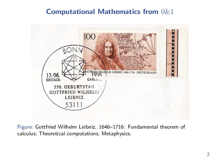
2. Computational Mathematics from 0&1 Figure: Gottfried Wilhelm Leibniz, 1646–1716: Fundamental theorem of calculus; Theoretical computations; Metaphysics. 2
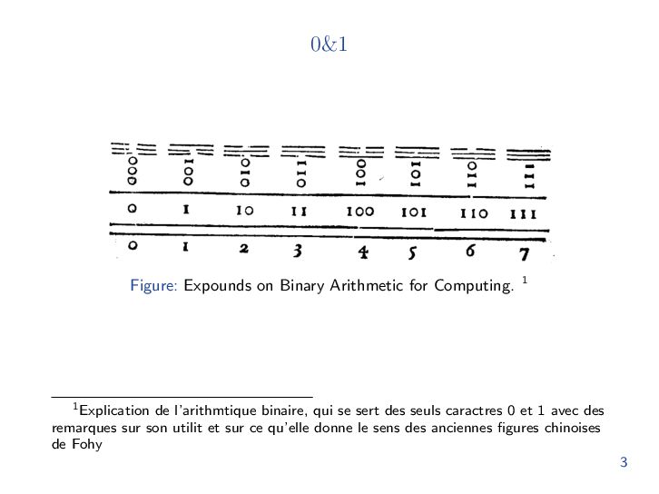
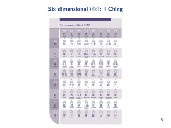
3. 0&1 Figure: Expounds on Binary Arithmetic for Computing. 1 1 Explication de l’arithmtique binaire, qui se sert des seuls caractres 0 et 1 avec des remarques sur son utilit et sur ce qu’elle donne le sens des anciennes figures chinoises de Fohy 3
4. Three dimensional 0&1 Figure: Philosophical Ising models 4
5. Six dimensional 0&1: I Ching 5
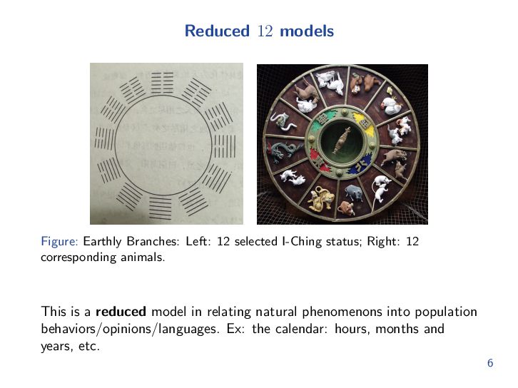
6. Reduced 12 models Figure: Earthly Branches: Left: 12 selected I-Ching status; Right: 12 corresponding animals. This is a reduced model in relating natural phenomenons into population behaviors/opinions/languages. Ex: the calendar: hours, months and years, etc. 6
7. Generative AI I Hopfield network and Restricted Boltzmann machines (Hinton, Hopfield, Amari, et.al.); I I Normalization flows and Neural ODEs (Chen, Ruthotto, et.al.); Generative adversarial networks (Goodfellow et.al.); I Stein variational gradient methods (Liu et.al.); I Di↵usion models (Song, Ermon et.al.); I Transformers for Natural Language models: Chat GPT (Illia et.al.); I ...... Can we understand and design AI algorithms in simulating and learning complex systems? 7
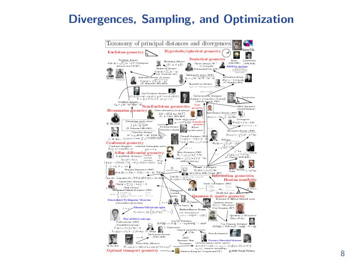
8. Divergences, Sampling, and Optimization Taxonomy of principal distances and divergences Euclidean geometry Hyperbolic/spherical geometry Euclidean distance !" d2 (p, q) = (p → qi )2 (Pythagoras’ i i theorem circa 500 BC) Hamming distance (|{i : pi ↑= qi }|) Euclid Pythagoras Manhattan "distance d1 (p, q) = i |pi → qi | (city block-taxi cab) Statistical geometry Physics #entropy JK →1 →k p log pdµ (Boltzmann-Gibbs 1878) Mahalanobis metric (1936) ! d! = (p → q)T !→1 (p → q) Minkowski distance !" (Lk -norm) dk (p, q) = k |pi → qi |k i (H. Minkowski 1864-1909) Bolyai (1802-1860) Lobachevsky (1792-1856) Additive entropy cross-entropy conditional entropy mutual information (chain rules) Information # entropy H(p) = → p log pdµ (C. Shannon 1948) Haussdorf set distance dH (X, Y ) = max{supx ϑ(x, Y ), supy ϑ(X, y)} H(p) = KL(p||u) Lévy-Prokhorov distance LPϖ (p, q) = inf ϱ>0 {p(A) ↔ q(Aϱ ) + ϱ↗A ↘ B(X )} Aϱ = {y ↘ X , ≃x ↘ A : ϑ(x, y) < ϱ} Quadratic distance ! dQ = (p → q)T Q(p → q) Lev M. Bregman Bhat. J.L. Koszul K. Nomizu % E. Vinberg ϖ 1 ω log J.M. Souriau Kullback-Leibler divergence # I-projection P KL(p||q) = p log pq dµ = Ep [log Q ] (relative entropy, 1951) Cone Je!rey divergence Non-Euclidean geometries geometry (Jensen-Shannon) Fisher information (local entropy) Riemannian geometry %ω &2 Bhattacharya distance (1967) I(ω) = E[ ωε ln p(X|ω) ] $# ↓ ↓ (R. A. Fisher 1890-1962) d(p, q) = → log p qdµ Finsler metric tensor Kolmogorov # 2 Riemannian metric tensor Symplectic gij = 12 ς 2 Fωyi(x,y) K(p||q) = |q → p|dµ ωy j # $ dxi dxj B. Riemann geometry gij ds ds ds (Kolmogorov-Smirnoff max |p → q|) Aitchison distance Hilbert ω = →1 (B. Riemann 1826-1866,) Probability simplex log-ratio metric Matsushita$ distance (1956) Fisher-Rao distance: # 1 1 ω 2 i j ↑ Mϑ (p, q) = |q ω → p ω |dµ ds = gij dω dω = Cherno! divergence (1952) # 1 !dω I(ω)dω # ˙ ↼(t)dt ˙ Cϑ (p||q) = → ln pϑ q 1→ϑ dµ C. R. Rao ϑF R (p, q) = minς 0 ↼(t)I(ω) Hellinger $# C(p, q) = maxϑ↓(0,1) Cϑ (p||q) ↓ ↓ Conformal geometry H(p||q) = ( p → q)2 ! ↓ Conformal divergence conformal Riemannian metric = 2(1 → f g ↑ω(1 → ω) D (p : q) = ϑ(p)D(p : q) g hi = eφ g p A!ne di”erential geometry Logarithmic divergence Constant sectional Pal & LG,ω (ϑ1 : ϑ2 ) =& curvature Wong 1 + ϖ→G(ϑ2 )↔ (ϑ1 ↓ ϑ2 ) +G(ϑ2 )↓G(ϑ1 ) 2016 ϖ ↔ 0, F = ↓G 2 Rényi divergence#(1961) 1 Hϑ = ϑ(1→ϑ) log f ϑ dµ # 1 Rϑ (p|q) = ϑ(ϑ→1) ln pϑ q 1→ϑ dµ (additive entropy) ϖ test # 2 Pearson ϖ2 (p||q) = (q→p) dµ p (K. Pearson, 1857-1936 ) ω = 0 ( Csiszár’ f -divergence # Df (p||q) = pf ( pq )dµ Vajda Neyman L. LeCam (Ali& Silvey 1966, Csiszár 1967) Information geometries Dual div.↓-conjugate (f ↓ (y) = yf (1/y)) Df ↓ (p||q) = Df (q||p) Hessian manifolds Bregman divergences (1967): Kullback-Leibler BF (ω1 ||ω2 ) = F (ω1 ) → F (ω2 ) → (ω1 → ω2 )↑ ↑F (ω2 ) Dual div. (Legendre) DF ↔ (↑F (ω1 )||↑F (ω2 )) = DF (ω2 ||ω1 ) Itakura-Saito divergence " IS(p|q) = i ( pqii → log pqii → 1) (Burg entropy) F. Itakura Bregman-Csiszár divergence (1991) ' Fω (x) = x → log x → 1 x log x → x + 1 1 (→xω + ωx → ω + 1) ω(1→ω) ω = 0 ω = 1 0 < ω < 1 Generalized Pythagoras’ theorem (Generalized projection) φ⇐ε Amari ε-divergence (1985) fω (x) = Generalized f -means duality... φ=1 Sharma-Mittal ) entropies * 1→ε %# ω & 1→ω 1 hω,ϖ (p) = 1↓ϖ p dµ ↓1 Non-additive entropy ' x log x → log x 4 (1 → x 1→ω2 1+ω 2 ) ω = 1 ω = →1 →1 < ω < 1 → Dually flat space Quantum & matrix geometry H. Shima →→ Fröbenius & Hilbert-Schmidt norm M. Nagumo B. De Finetti Burbea-Rao or Jensen (incl. Jensen-Shannon) JF (p; q) = f (p)+f (q) →f 2 % p+q & 2 Quantum entropy S(ϑ) = →kTr(ϑ log ϑ) (Von Neumann 1927) Quantum f -divergences (Dénes Petz) J. Jensen Log Det divergence D(P||Q) =< P, Q→1 > → log det PQ→1 → dimP Von Neumann divergence D(P||Q) = Tr(P(log P → log Q) → P + Q) L. Kantorovich # pω Integral probability metrics 1 Tϑ (p||q) = 1→ϑ (1 → qω→1 dµ) G. Monge IPMs Stein discrepancies Earth mover distance (EMD 1998) ϑ = L1 MMD Gromov-Haussdorf distance Maximum Mean (between compact metric spaces) Discrepancy Wasserstein distances 1 dGH (X, Y ) = inf φX :X↗Z,φY :Y ↗Z {ϑZ M. Fréchet H (↽X (X), ↽Y (Y ))} Wω,ε (p, q) = (inf ϑ↑!(p,q) ω(p, q)ω dε(x, y)) ω ↽X , ↽Y : isometric embeddings Optimal transport geometry 2023 Frank Nielsen Sinkhorn divergence (h-regularized OT) Tsallis entropy (1998) (Non-additive # entropy) 1 Tϑ (p) = 1→ϑ ( pϑ dµ → 1) 8
9. Transport information geometry Main Question: Analyzing and constructing AI type numerical methods for simulating complex systems. Physics and computations I Wasserstein efficiency (Amari, Li, Matsuda, Zhao, Rubio ...) I Wasserstein natural gradient (Li, Montufar, Osher, Chen, Lin, Abel, Liu ...) I Wasserstein divergences (Wang, Pal, Guo, Li, Ay ...) I Minimal Wasserstein surfaces (Georgiou, Li, ...) I Wasserstein fluctuation and non-equilibrium thermodynamics (Ito, Kobayashi, Li, Liu, Gao ...) I Wasserstein di↵usions and Dean-Kawasaki dynamics (Renesse, Sturm, Li ...) I Stochastic Dynamical density functional theory (SDDFT). 9
10. Current studies in 2026-2027 I Sparse Transformer Architectures via Regularized Wasserstein Proximal Operator with L1 Prior; I Sympformer: accelerated attention blocks via inertial dynamics on density manifolds; I Natural gradient in solving mean field control problems; I Continue studies for score-based neural ODEs in simulating Fokker-Planck equations; I Construction of Wasserstein di↵usions on simplex sets; 10
11. Sparse Transformer Architectures via Regularized Wasserstein Proximal Operator with L1 Prior Fuqun Han, Stanley Osher, Wuchen Li arXiv 2510.16356 (2025)
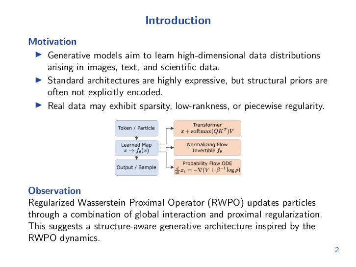
12. Introduction Motivation ↭ Generative models aim to learn high-dimensional data distributions arising in images, text, and scientific data. ↭ Standard architectures are highly expressive, but structural priors are often not explicitly encoded. ↭ Real data may exhibit sparsity, low-rankness, or piecewise regularity. Observation Regularized Wasserstein Proximal Operator (RWPO) updates particles through a combination of global interaction and proximal regularization. This suggests a structure-aware generative architecture inspired by the RWPO dynamics. 2
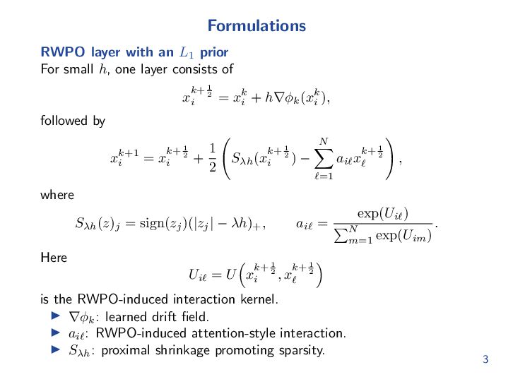
13. Formulations RWPO layer with an L1 prior For small h, one layer consists of k+ 12 xi followed by 1 k+ 1 xk+1 = xi 2 + i 2 = xki + h→ωk (xki ), ! k+ 1 Sωh (xi 2 ) ↑ where Sωh (z)j = sign(zj )(|zj | ↑ εh)+ , Here N " k+ 1 aiε xε 2 ε=1 # , exp(Uiε ) aiε = $N . m=1 exp(Uim ) % & k+ 1 k+ 1 Uiε = U xi 2 , xε 2 is the RWPO-induced interaction kernel. ↭ →ωk : learned drift field. ↭ aiε : RWPO-induced attention-style interaction. ↭ Sωh : proximal shrinkage promoting sparsity. 3
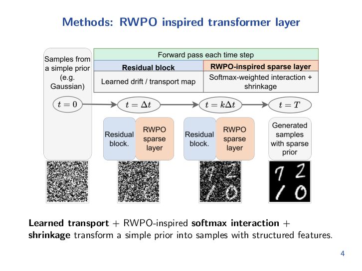
14. Methods: RWPO inspired transformer layer Learned transport + RWPO-inspired softmax interaction + shrinkage transform a simple prior into samples with structured features. 4
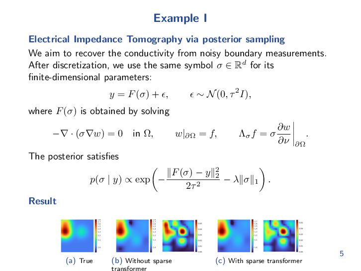
15. Example I Electrical Impedance Tomography via posterior sampling We aim to recover the conductivity from noisy boundary measurements. After discretization, we use the same symbol ϑ ↔ Rd for its finite-dimensional parameters: y = F (ϑ) + ϖ, where F (ϑ) is obtained by solving ↑→ · (ϑ→w) = 0 in !, The posterior satisfies Result ϖ ↗ N (0, ϱ 2 I), w|ϑ! = f, ' ςw '' ”ϖ f = ϑ . ςφ 'ϑ! ( ) ≃F (ϑ) ↑ y≃22 p(ϑ | y) ↘ exp ↑ ↑ ε≃ϑ≃ 1 . 2ϱ 2 (a) True (b) Without sparse transformer (c) With sparse transformer 5
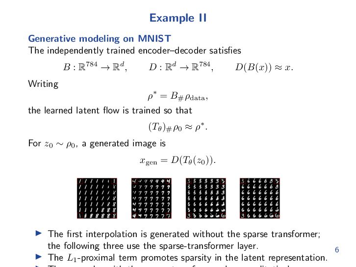
16. Example II Generative modeling on MNIST The independently trained encoder–decoder satisfies Writing B : R784 ⇐ Rd , D : Rd ⇐ R784 , D(B(x)) ⇒ x. ↼→ = B# ↼data , the learned latent flow is trained so that (Tϱ )# ↼0 ⇒ ↼→ . For z0 ↗ ↼0 , a generated image is xgen = D(Tϱ (z0 )). ↭ The first interpolation is generated without the sparse transformer; the following three use the sparse-transformer layer. 6 ↭ The L1 -proximal term promotes sparsity in the latent representation.
17. Papers along this direction ↭ Fuqun Han, Stanley Osher, and Wuchen Li, Tensor Train Based Sampling Algorithms for Approximating Regularized Wasserstein Proximal Operators, SIAM/ASA J. Uncertain. Quantif., 13 (2025), 775–804. ↭ Fuqun Han, Stanley Osher, and Wuchen Li, Convergence of Noise-Free Sampling Algorithms with Regularized Wasserstein Proximals, J. Mach. Learn. Res., 27(85) (2026), 1–66. ↭ Fuqun Han, Stanley Osher, and Wuchen Li, Splitting Regularized Wasserstein Proximal Algorithms for Nonsmooth Sampling Problems, arXiv:2502.16773, 2025. ↭ Fuqun Han, Stanley Osher, and Wuchen Li, Sparse Transformer Architectures via Regularized Wasserstein Proximal Operator with L1 Prior, arXiv:2510.16356, 2025. 7
18. SympFormer: Accelerated attention blocks via Inertial Dynamics on Density Manifolds Viktor Stein, Wuchen Li, Levin Maier, Gabriele Steidl https://arxiv.org/abs/2603.16535
19. Transformer architecture [7] stacked decoder-like sublayers, made up of I (masked multi-head) self-attention I token-wise feed-forward neural networks (aka MLP) with residual (aka skip connections) I (layer normalization) Figure: Autoregressive decoder-only transformer architecture (GPT). Figure modified from [5]. (Variant of encoder-decoder transformer “T5”) Training via backpropagation: loss = predict next token given the previous ones. Generation: predict next token, add to rest (”context”), repeat (”autoregression”) 2
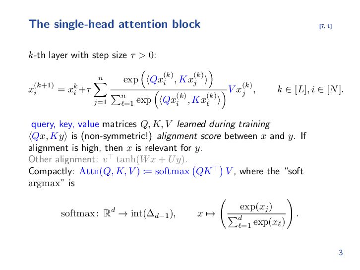
20. The single-head attention block k-th layer with step size ⌧ > 0: ⇣ ⌘ (k) (k) n exp hQxi , Kxj i X (k+1) ⇣ ⌘ V x(k) xi = xki +⌧ j , Pn (k) (k) exp hQx , Kx i j=1 i `=1 ` [7, 1] k 2 [L], i 2 [N ]. query, key, value matrices Q, K, V learned during training hQx, Kyi is (non-symmetric!) alignment score between x and y. If alignment is high, then x is relevant for y. Other alignment: v > tanh(W x + U y). Compactly: Attn(Q, K, V ) := softmax QK > V , where the “soft argmax” is ! exp(xj ) d softmax : R ! int( d 1 ), x 7! Pd . `=1 exp(x` ) 3
21. The attention ODE [4, 8] From now on: ignore normalization & MLP. Each transformer sublayer = one discrete time step. Letting the step size ⌧ ! 0 (like in neural ODEs), we obtain (unmasked single-head) self-attention ẋi (t) = n X exp (hQxi (t), Kxj (t)i) Pn V xj (t), `=1 exp (hQxi (t), Kx` (t)i) j=1 i 2 [n], t > 0. (1) xi (t) - tokens or representations at time t, (1) is a simplified version of forward pass through the infinitely deep trained transformer with the same Q, K, V in all layers (“weight sharing”). 4
22. Mean field limit - the transformer PDE [2, 3] Mean field limit of infinitely many tokens: n {xi }ni=1 ! 1X n!1 ! µ 2 P(Rd ) x n i=1 i On probability measures P(Rd ), the transformer ODE becomes the transformer PDE Z exp (hQx, Kyi) µ̇t = r· µt (µt ) , [ (µ)](x) := V yR dµ(y) exp (hQx, Kzi) dµ(z) d Rd R (2) called softmax attention mapping. (2) is a gradient flow of ZZ 1 SM := F (⇢) exp(y > Ax)⇢(x)⇢(y) dx dy, A := Q> K 2 in the non-linear mobility Wasserstein geometry, given by G⇢ 1 [ ] := r · ( (⇢)r ), where (⇢)(x) := R exp(z>⇢(x) B, Ax)⇢(z) dz B := V A 1 . 5
23. SympFormer - an accelerated transformer [6] We consider the accelerated variant of the transformer PDE. Lemma (Accelerated softmax attention PDE) The accelerated softmax attention flow satisfies ✓ ◆ 8 Br t (x) > R > @t ⇢t (x) + r · ⇢t (x) = 0, > > exp (z > Ax) ⇢t (z) dz > > > 2 < kr t (x)kB 1 @t t (x) + (t) t (x) + R 2 exp (z > Ax) ⇢t (z) dz > ! > Z > > 1 kr t (y)kB 2 > > > > exp y Ax R : 2 + 2 ⇢t (y) dy = 0. 2 exp (z > Ay) ⇢t (z) dz (3) PN 1 A particle discretization ⇢t ⇡ N k=1 Xk (t) yields, in matrix form, ( Ẋ(t) = N diag(M(t) ) 1 Y(t)B > , (4) Ẏ(t) = (t)Y(t) + N2 {R(t), M(t)} + 2M(t) X(t)A, where Yi (t) := r t (Xi (t)), Mi,j (t) := exp Xi (t)> AXj (t) , and R depends on Y, M, and B. 6
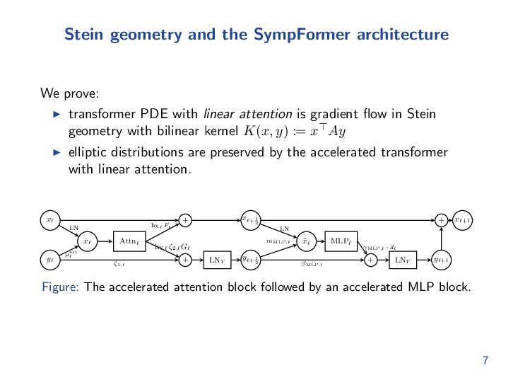
24. Stein geometry and the SympFormer architecture We prove: I transformer PDE with linear attention is gradient flow in Stein geometry with bilinear kernel K(x, y) := x> Ay I elliptic distributions are preserved by the accelerated transformer with linear attention. x` h X ` F` LN x̄` y` Attn` µatt ` ⇣1,` x`+ 1 + + 2 x`+1 LN mMLP,` hY ` ⇣2,` G` + LNY x̃` y`+ 1 2 MLP,` MLP` MLP,` · d` + LNY y`+1 Figure: The accelerated attention block followed by an accelerated MLP block. 7
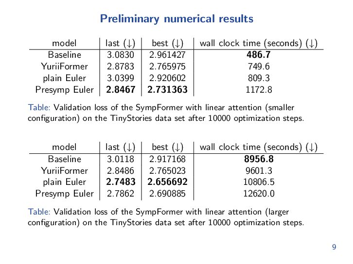
25. Preliminary numerical results model Baseline YuriiFormer plain Euler Presymp Euler last (#) 3.0830 2.8783 3.0399 2.8467 best (#) 2.961427 2.765975 2.920602 2.731363 wall clock time (seconds) (#) 486.7 749.6 809.3 1172.8 Table: Validation loss of the SympFormer with linear attention (smaller configuration) on the TinyStories data set after 10000 optimization steps. model Baseline YuriiFormer plain Euler Presymp Euler last (#) 3.0118 2.8486 2.7483 2.7862 best (#) 2.917168 2.765023 2.656692 2.690885 wall clock time (seconds) (#) 8956.8 9601.3 10806.5 12620.0 Table: Validation loss of the SympFormer with linear attention (larger configuration) on the TinyStories data set after 10000 optimization steps. 9
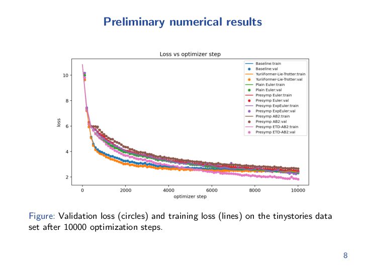
26. Preliminary numerical results Figure: Validation loss (circles) and training loss (lines) on the tinystories data set after 10000 optimization steps. 8
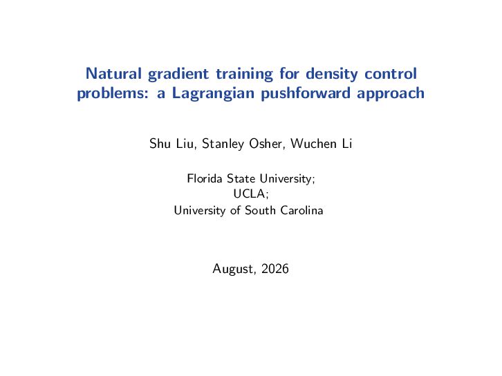
27. Natural gradient training for density control problems: a Lagrangian pushforward approach Shu Liu, Stanley Osher, Wuchen Li Florida State University; UCLA; University of South Carolina August, 2026
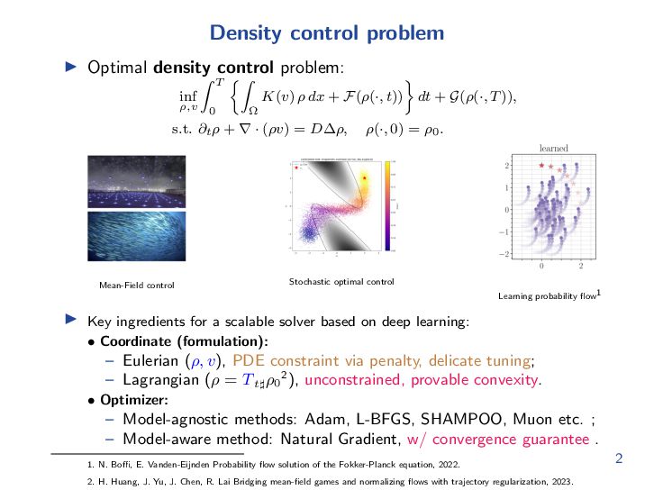
28. Density control problem ↭ Optimal density control problem: inf ω,v ! T "! 0 ! # K(v) ω dx + F (ω(·, t)) dt + G(ω(·, T )), s.t. εt ω + → · (ωv) = D!ω, Mean-Field control ω(·, 0) = ω0 . Stochastic optimal control Learning probability flow1 ↭ Key ingredients for a scalable solver based on deep learning: • Coordinate (formulation): – Eulerian (ω, v), PDE constraint via penalty, delicate tuning; – Lagrangian (ω = T tε ω0 2 ), unconstrained, provable convexity. • Optimizer: – Model-agnostic methods: Adam, L-BFGS, SHAMPOO, Muon etc. ; – Model-aware method: Natural Gradient, w/ convergence guarantee . 1. N. Bo!, E. Vanden-Eijnden Probability flow solution of the Fokker-Planck equation, 2022. 2. H. Huang, J. Yu, J. Chen, R. Lai Bridging mean-field games and normalizing flows with trajectory regularization, 2023. 2
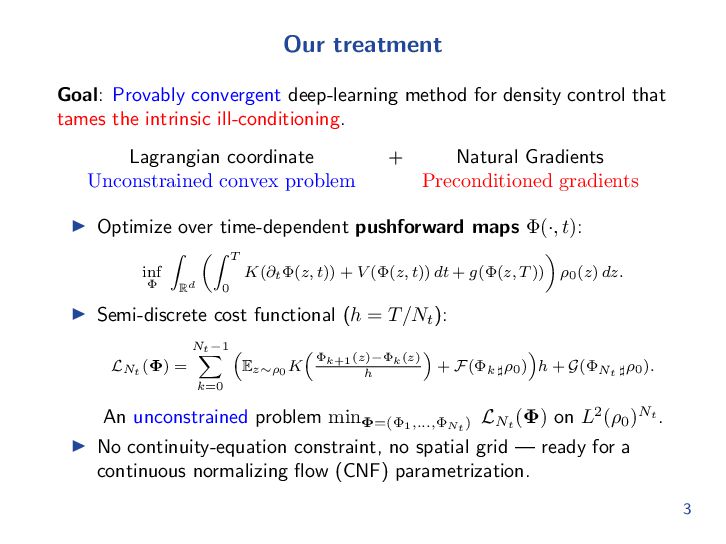
29. Our treatment Goal: Provably convergent deep-learning method for density control that tames the intrinsic ill-conditioning. Lagrangian coordinate Unconstrained convex problem + Natural Gradients Preconditioned gradients ↭ Optimize over time-dependent pushforward maps !(·, t): inf ” ! $! T % K(εt ”(z, t)) + V (”(z, t)) dt + g(”(z, T )) ω0 (z) dz. N& t →1 ' Ez↑ω0 K Rd 0 ↭ Semi-discrete cost functional (h = T /Nt ): LNt (!) = k=0 ' ”k+1 (z)→”k (z) h ( ( + F (”k ε ω0 ) h + G(”Nt ε ω0 ). An unconstrained problem min!=(!1 ,...,!Nt ) LNt (!) on L2 (ω0 )Nt . ↭ No continuity-equation constraint, no spatial grid — ready for a continuous normalizing flow (CNF) parametrization. 3
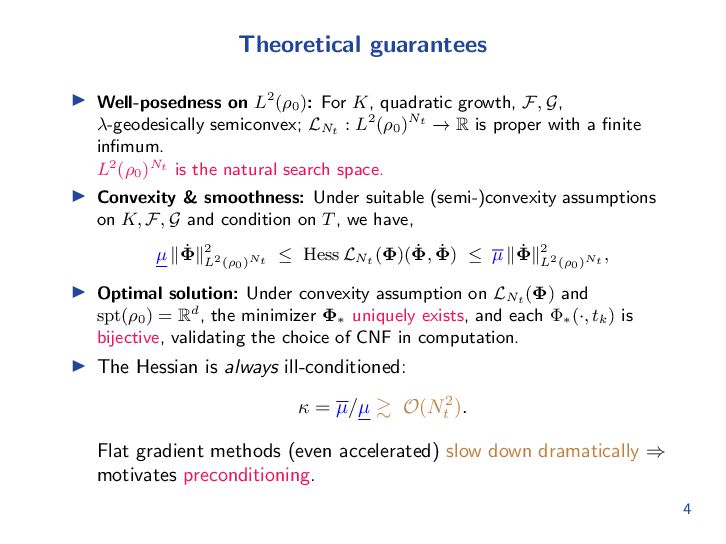
30. Theoretical guarantees ↭ Well-posedness on L2 (ω0 ): For K, quadratic growth, F , G, ε-geodesically semiconvex; LNt : L2 (ω0 )Nt → R is proper with a finite infimum. L2 (ω0 )Nt is the natural search space. ↭ Convexity & smoothness: Under suitable (semi-)convexity assumptions on K, F , G and condition on T , we have, ˙ 22 ˙ ˙ ˙ 2 µ ↑!↑ L (ω0 )Nt ↓ Hess LNt (!)(!, !) ↓ µ ↑!↑L2 (ω0 )Nt , ↭ Optimal solution: Under convexity assumption on LNt (!) and spt(ω0 ) = Rd , the minimizer !↓ uniquely exists, and each !↓ (·, tk ) is bijective, validating the choice of CNF in computation. ↭ The Hessian is always ill-conditioned: ε = µ/µ ↫ O(Nt2 ). Flat gradient methods (even accelerated) slow down dramatically → motivates preconditioning. 4
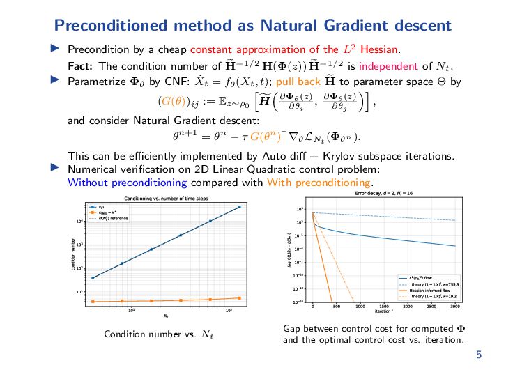
31. Preconditioned method as Natural Gradient descent ↭ Precondition by a cheap constant approximation of the L2 Hessian. ) →1/2 H(!(z)) H ) →1/2 is independent of Nt . Fact: The condition number of H ) to parameter space # by ↭ Parametrize !ϑ by CNF: Ẋt = fϑ (Xt , t); pull back H * ' (, + ϖ!ω (z) , ϖ!ω (z) , (G(ϑ))ij := Ez↑ω0 H ϖϑ ϖϑ i j and consider Natural Gradient descent: ϑ n+1 = ϑ n ↑ ϖ G(ϑn )† →ϑ LNt (!ϑn ). This can be e!ciently implemented by Auto-di” + Krylov subspace iterations. ↭ Numerical verification on 2D Linear Quadratic control problem: Without preconditioning compared with With preconditioning. Condition number vs. Nt Gap between control cost for computed ! and the optimal control cost vs. iteration. 5
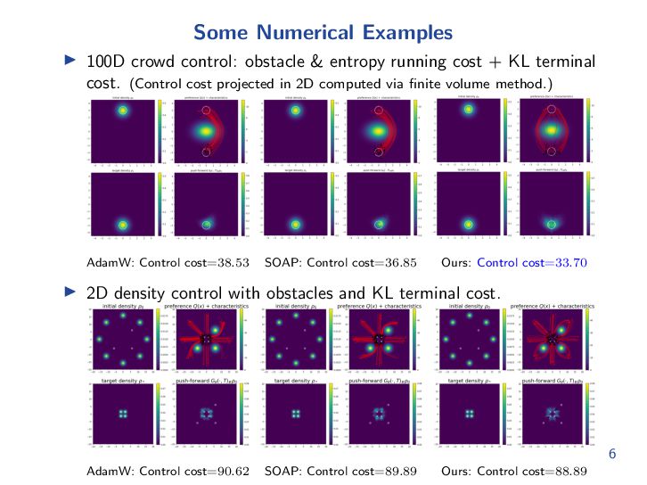
32. Some Numerical Examples ↭ 100D crowd control: obstacle & entropy running cost + KL terminal cost. (Control cost projected in 2D computed via finite volume method.) AdamW: Control cost=38.53 SOAP: Control cost=36.85 Ours: Control cost=33.70 ↭ 2D density control with obstacles and KL terminal cost. 6 AdamW: Control cost=90.62 SOAP: Control cost=89.89 Ours: Control cost=88.89
33. Related publications 1. Shu Liu, Siting Liu, Stanley Osher, Wuchen Li. A first-order computational method for Reaction-Di”usion type equations via Primal-Dual Hybrid Gradient method. Journal of Computational Physics (JCP), Volume 500, 2024. 2. Shu Liu, Xinzhe Zuo, Stanley Osher, Wuchen Li. Numerical analysis of a first-order computational algorithm for reaction-di”usion equations via the primal-dual hybrid gradient method. Mathematics of Computation (Math. Comp.), July 11, 2025. 3. Shu Liu, Stanley Osher, Wuchen Li. A Natural Primal-Dual Hybrid Gradient Method for Adversarial Neural Network Training on Solving Partial Di”erential Equations. Accepted by JMLR. 4. Shu Liu, Stanley Osher, Wuchen Li. Natural gradient training for density control problems: a Lagrangian pushforward approach. Preprint in preparation. 7
34. Simulating Fokker–Planck equations via mean field control of score-based normalizing flows Mo Zhou Stanley Osher Wuchen Li Aug, 2026 arxiv.org/abs/2506.05723
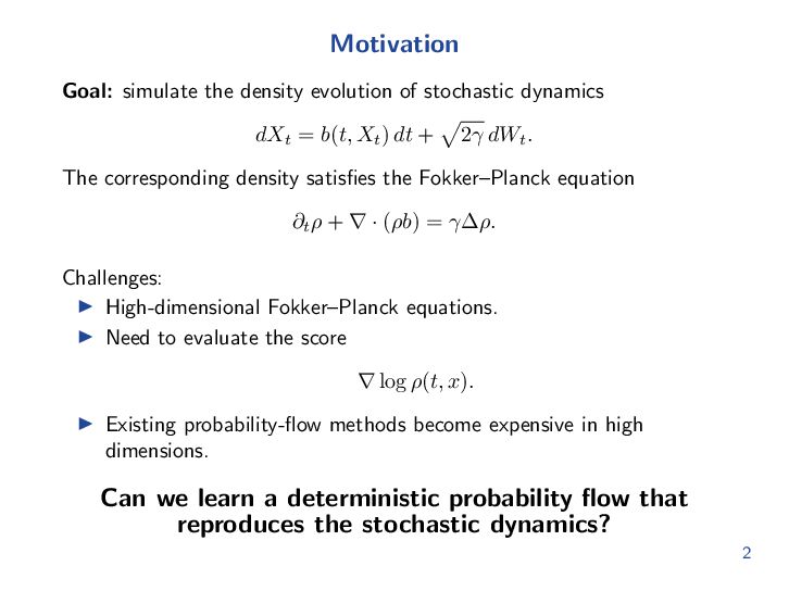
35. Motivation Goal: simulate the density evolution of stochastic dynamics ! dXt = b(t, Xt ) dt + 2ω dWt . The corresponding density satisfies the Fokker–Planck equation εt ϑ + → · (ϑb) = ω!ϑ. Challenges: ↭ High-dimensional Fokker–Planck equations. ↭ Need to evaluate the score → log ϑ(t, x). ↭ Existing probability-flow methods become expensive in high dimensions. Can we learn a deterministic probability flow that reproduces the stochastic dynamics? 2
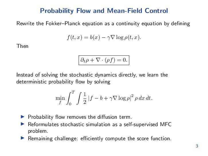
36. Probability Flow and Mean-Field Control Rewrite the Fokker–Planck equation as a continuity equation by defining f (t, x) = b(x) ↑ ω→ log ϑ(t, x). Then εt ϑ + → · (ϑf ) = 0. Instead of solving the stochastic dynamics directly, we learn the deterministic probability flow by solving min f " T" 0 1 2 |f ↑ b + ω→ log ϑ| ϑ dx dt. 2 ↭ Probability flow removes the di!usion term. ↭ Reformulates stochastic simulation as a self-supervised MFC problem. ↭ Remaining challenge: e”ciently compute the score function. 3
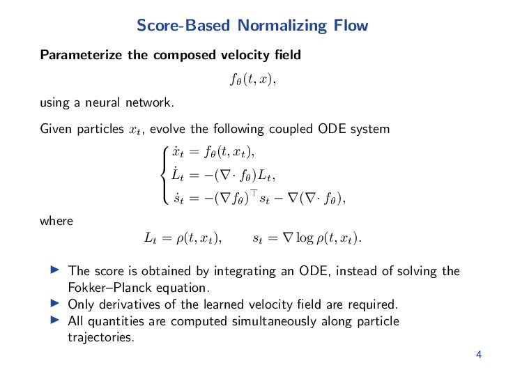
37. Score-Based Normalizing Flow Parameterize the composed velocity field fω (t, x), using a neural network. Given particles xt , evolve the following coupled ODE system  ẋ = fω (t, xt ),   t L̇t = ↑(→· fω )Lt ,   ṡt = ↑(→fω )→ st ↑ →(→· fω ), where Lt = ϑ(t, xt ), st = → log ϑ(t, xt ). ↭ The score is obtained by integrating an ODE, instead of solving the Fokker–Planck equation. ↭ Only derivatives of the learned velocity field are required. ↭ All quantities are computed simultaneously along particle trajectories. 4
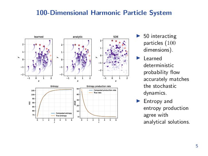
38. 100-Dimensional Harmonic Particle System ↭ 50 interacting particles (100 dimensions). ↭ Learned deterministic probability flow accurately matches the stochastic dynamics. ↭ Entropy and entropy production agree with analytical solutions. 5
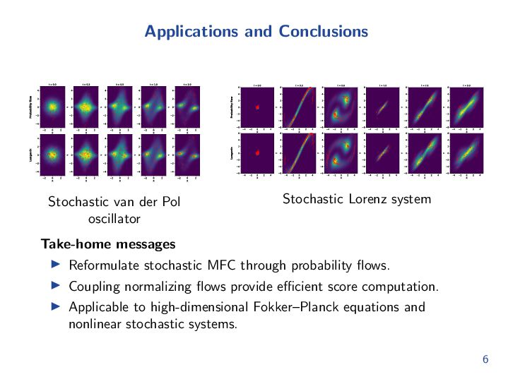
39. Applications and Conclusions Stochastic van der Pol oscillator Stochastic Lorenz system Take-home messages ↭ Reformulate stochastic MFC through probability flows. ↭ Coupling normalizing flows provide e”cient score computation. ↭ Applicable to high-dimensional Fokker–Planck equations and nonlinear stochastic systems. 6
40. Related Work on Score-Based Mean-Field Control Forward–Backward Score Dynamics (Res. Math. Sci., 2025) Score-based neural ODE (JCP, 2025) This work (JCP, 2026) ↭ Learn the probability flow by parameterizing the velocity field. ↭ E!cient simulation of high-dimensional Fokker–Planck equations. Variational Conditional Normalizing Flow (under review) 7
41. Future work I Analyze information matrices and divergences for Scientific machine learning problems; I Build kinetic information matrices for kinetic simulations; I Develop information matrices for approximating stochastic DDFT; I Design quantum information matrices for quantum computing problems. I ...... Thanks for the continuous support from Fariba and AFOSR! 11