Photometric Image Processing for HDR Displays

Many real-world scenes contain a dynamic range that exceeds conventional display technology by several orders of magnitude. Through the combination of several existing technologies, new high dynamic range displays, capable of reproducing a range of intensities much closer to that of real environments, have been constructed. These benefits come at the cost of more optically complex devices; involving two image modulators, controlled in unison, to display images. We present several methods of rendering images to this new class of devices for reproducing photometrically accurate images. We discuss the process of calibrating a display, matching the response of the device with our ideal model. We then derive series of methods for efficiently displaying images, optimized for different criteria and evaluate them in a perceptual framework.

Transcript

1. Photometric Image Processing for High Dynamic Range Displays Matthew Trentacoste University of British Columbia
2. Introduction • High dynamic range (HDR) imaging – Techniques that can store and manipulate images with higher bit depths – Able to accommodate images that are brighter, have more contrast, and are more accurate than conventional images – Opens up new possibilities • Desire to display this additional data – Can tone map, and apply some function that remaps pixel values to better preserve the impression – Much is lost -- some image information, and the viceral experience of the original scene is not conveyed – The reason we don’t confuse a photograph of a car and headlights at night with the real thing – Inherently low dynamic range (LDR) means of display cannot convey what we want, and motivates other means
3. HDR displays • Overcome hardware constraints – No single material is capable of simultaneously reproducing the luminances, bit depths, resolutions, and form factors required for displaying HDR images – The limited contrast of LCD panel requires an additional modulator – Replace the uniform light behind the LCD panel with a low resolution, high contrast display – Many options, and either a projector or grid of ultra-bright LEDs is used in practice • Many benefits, but equally as many challenges – Pixels are no longer independent, altering the backlight to adjust the luminance at one pixel causes a luminance change at other pixels – Cannot exactly reproduce the luminances of real scenes – More complicated techniques required to display images
4. Image processing for HDR displays • Challenge : – Given an image, compute a matched set of front and back images that combined by the display optics produce the same observed image as the original • Show this is possible – Even with inexact reproduction of hardware – Shortcomings of human perception – Processing can be performed efficiently • Full realization beyond the scope of a single thesis – Much of the perceptual foundation is not completely explored – Only address the accurate reproduction of perceived luminances
5. Outline • Related work • Processing algorithms • Measurement and calibration • Evaluation • Conclusion
6. Related work • Perception and psychophysics – Basis of assumptions in hardware and software design – Critical role in ensuring claims of image quality • Tone mapping operators – Work on displaying HDR images without resorting to HDR display • HDR technology – Foundations and physical make-up – Serves as a starting platform for all of our contributions • Display calibration – Review LDR techniques for comparison – What is required for accurate HDR image presentation
7. Perception • Simple metrics fail to capture the complexity of human vision, and a study of perception is required – Body of research on HVS
   
   
   larger than the scope here – Focus on several topics pertinent to HDR image display • Local contrast perception – Quality and impact of the optics of the eye on how we see • Luminance quantization – Sensitivity to changes in light • Visible difference prediction – Modeling of HVS to predict which image artifacts are likely noticed
8. Local contrast perception • Limits on what contrasts we can accurately perceive – Ocular scatter obscures details on the darker side of high contrast edges – Maximum perceived contrast around 150:1 – Well documented [Moon 1944,1945] [Vos 1986] [Deeley 1991] • Key element of HDR display effectiveness – Exploits inability to see detail in vicinity of high contrast boundaries – Relative and absolute luminances maintained – Only when boundary exceeds contrast of LCD panel is there a loss of fidelity
9. Luminance quantization • Human eye does not respond linearly to luminance – HVS much more sensitive to changes at luminances – For low intensity Yd and high intensity Yb and some change ∆Y the perceived change between Yd and Yd +∆Y is greater than Yb and Yb +∆Y – Numerous studies [Blackwell 1981] [Ferwerda 1996] – Described in terms of threshold vs intensity (TVI), the smallest detectable change at a luminance level – Commonly referred to as just noticeable differences - the unit of perceptually uniform lightness – Ploted as contrast vs intensity (CVI) the ratio of the same term
10. Just noticeable differences • JND defines a step of the luminance scale – The smallest detectable difference at a given luminance level – Anything less is not perceptually relevant • Important consideration in imaging system design – Providing additional driving values in the space of 1 JND is redundant • HDR luminance quantizations – [DICOM 2001] is based on contrast sensitivity studies [Barten 1992] – [Mantiuk 2004] is based on solving TVI measurements for the mapping functions
11. Visible difference prediction • Common metrics such as least squares poor estimates of perceived differences – Not representative of the complex mechanisms that comprise the HVS • Visible differences – Schemes exist to address this [Daly 1993] [Lubin 1995] – Explicitly model aspects of early vision to yield better evaluations • HVS model – Start with the two aspects we mentioned, ocular scatter and lightness – Add in subsequent portions of the visual pathways that model detection mechanisms in the brain • As of current, only 1 HDR VDP [Mantiuk 2005] – Modification of Daly to handle larger ranges of luminances
12. HDR VDP Mantiuk HDR VDP 1. Apply the ocular scattering to both images 2. Apply lightness sensitivity 3. Apply a function that models our contrast sensitivity 4. Filter by frequency+orientation like visual cortex 5. Weight and sum up probabilities to produce map
13. Tone mapping operators • Remap scene luminances to displayable values – Preserve the impression of the original image – Traditional method of displaying HDR images (paintings, photographs) – Only method before HDR displays were available – Body of work too large to cover here, see [Reinhard 2005] • Pertinent operators – [Durand 2002] separates the image into a base luminance layer and a detail layer, similar to a stage of our work – [Chiu 1993] divides the original image by a blurred version of it, discarding large luminance differences while retaining detail but causes undesireable “reverse gradients” around bright objects – We perform a similar operation to account for the display optical package, but we are use to use the resulting gradients to our advantage
14. Shortcomings of tone mapping • Cannot represent all information – Can depict more information than linear scaling, but still limited – The HDR display luminance range contains roughly 1000 JNDs – Most conventional media are only 8-bit and preserve 25% of the data • Luminance-dependent experiences – There are perceptual and psychophysical effects that depend on luminance alone – Tone mapping can show detail in all areas of an image of a car and headlights at night but no one would confuse it for the original – Operators can mimic processes of the HVS to deliver more information, but they cannot reproduce the visceral experiences of the original scene illumination
15. HDR technology • Conventional LCDs – Consist of a liquid crystal modulating a uniform backlight – Important to note that LCDs can’t completely block light transmission – The ratio of the peak intensity to this light leakage is the dynamic range – Can increase backlight intensity, but dynamic range is still limiting factor • HDR displays use an LCD panel as an optical filter – Programmable transparency modulates a high intensity but low resolution image from a second display – If contrast ratio of LCD is c1 : 1 and other display is c2 : 1, then the (theoretical) contrast ratio of the HDR display is ( c1 * c2 ) : 1 • Two versions built on this concept – Display based on a projector – Display based on a grid of LEDs
16. Projector-based display • Three primary components – Projector, LCD, and coupling optics • Alignment issues – Single housing with alignment mechanisms, but perfect alignment is still near impossible – To avoid moiré patterns and artifacts associated with even a slight misalignment – Purposefully blur projector image, and compensate for in processing • Specifications – Dynamic range of 54,000 : 1 – Luminance range from 0.05 cd/m2 to 2700 cd/m2 – 962 JND values, and over 17,000 unique driving values
17. LED-based display • Overcome projector issues – Power, thermal management, and form factor all infeasible for a product • Backlight resolution – Possible to compensate for the low resolution of the rear image – Correction works perfectly as long as local image contrast does not exceed dynamic range of LCD – From the model of ocular scatter, can establish a maximum size for a rear image pixel • BRIGHTSIDE DR-37P – 4760 cd/m2 for a full white center square, and a minimum luminance of less than 6 cd/m2 on ANSI 9 checkerboard, yielding 875 JNDs
18. Display Calibration
19. Challenges in image display Challenge 1 • Map an image containing luminances or colors that exceed the capabilities of the monitor into the color space of display • Convert a scene-referred image into an output-referred image Challenge 2 • To process image data for display, taking image intensities and a gamut within that of the display and producing the best possible image • Convert an output-referred image to actual luminances
20. Processing Algorithms • Work here only addresses the second challenge – Given meaningful data, we want to display the best image possible • Reference algorithm – High-level view of the problem being considered • Performance-related modifications – Altering the reference method to be feasible • Implementation – Step-by-step description of the actual methods used in practice • Error diffusion – Additional final process to improve results
21. Reference Algorithm Nonlinear optimization problem – Make as few assumptions as possible – Compare displayed image to desired image using perceptually- based objective Required components – Simulation of display hardware – Perceptual transformation – Objective function + constraints – Numerical solver
22. Display hardware simulation • Take in driving values on the range [0,1] and map them to measured photometric units • Need to have the shape of the blur, also called pointspread function (PSF), performed by the diffuser • Model as a 2D convolution of a set of Dirac delta functions at the locations of the LEDs by the diffuser PSF • In the set δ D each LED δ j is modulated by a driving value dj giving • where I is the simulated image, p is the values of the LCD panel, and PSFD is the Gaussian fitting the PSF
23. Perceptual transform • Employ function similar to the VDP • Use simplified model that only includes ocular scatter and perceived lightness • To simplify further, ignoring all detection mechanisms and have the function • where PSFe is the pointspread function of the human eye at adaptation luminance Yavg , and L is the luminance quantization in JND units
24. Observations • Objective function is then the least squares error between the perceptual transformed versions of both the desired image and the simulation • The constraints address 2 issues – The values are physically plausible ie. p,d 㱨
    [0,1] – The total power draw of the LEDs is less than some amount so that the breaker isn’t blown – where e is the power consumed by an LED at full and etot is the maximum power • Can be solved with any number of NLLS solvers
25. Observation sample • Original (left) • Backlight (center) is a low-frequency version of the original • LCD (right) contains the remaining image content, adjusted for the backlight
26. Performance-related modifications • Major disadvantage to the reference algorithm – Slow : large iterative methods, can take hours • Precomputation infeasible in most applications – A monitor is expected to display images in real-time – The base requirement of 60Hz implies the algorithm completes its work in under 12.5ms using available computational resources, like a GPU or FPGA • Must improve performance – Take advantage of problem structure – Reduce complexity of functions used, size of the systems involved, number of iterations • Start by discarding perceptual transform – Too computationally intensive for real-time, but still of use for validation
27. Simplification of simulation • Simulation function structure enforced by hardware – Original image is distributed between the LCD and LEDs – The LCD panel compensates for the low frequency of the backlight • Simulation a linear system – PSFD constant for a given LED layout and diffuser, and can be precomputed and this is equivalent to the system – tied together by the n x m weighting matrix W which accounts for the layout of the LEDs and the PSF of the diffuser – Where m = # pixels and n = # LEDs
28. Problem decomposition • Linear independence of LCD pixels • Break problem down into 2 sequential steps • Solve for the LED values • Create the matching LCD image trivially by back substitution (division) to find the values that best approximate for a given backlight • Given backlight B = Wd then • and is seen to the right Original Backlight Corrected
29. Target Backlight • Separation of backlight and LCD – Must be able to determine target backlight from the desired image I’ • Consider idealized projector version – Assume projector and LCD are linear and have the same dynamic range – Also ignore alignment and blurring of the projector image – Under these assumptions, the target image I’ could be achieved by normalizing the values and taking the square root – Target backlight is the sqrt of the desired image • Possible to decouple – Deconvolution that determines LEDs and simulation that determines the matching LCD image can be performed separately – Reduces m x m + n system to 2 m x n systems – Significant speedup since m ≈ 1000 x n
30. Approximate solution • Approximate method speedups – No longer guarantee the exact solution, but sufficiently close • Low spatial frequency of backlight – Can downsample to a lower resolution without measurable change – Less elements to solve for in deconvolution stage and less to iterate over in simulation stages • No longer required to iterate – Besides producing the desired image, the LCD and LED values must accurately match each other – Previously required solver convergence to guarantee match – LCD is now matched to backlight by definition, iteration is optional
31. Implementation • How to perform in practice • 4 steps – Given the desired image I’, determine the target backlight B’ – Determine the LED driving values d that best approximate B’ – Given d, simulate the resulting backlight B – Determine the LCD panel p that corrects for the low frequency of the backlight
32. Sample image
33. Target backlight • Takes desired image I’ and produces the target backlight B’ • Both input and output are in photometric units • Clamp to maximum display value, Imax • Divide up the dynamic range between the two displays by taking sqrt • Downsample to lower resolution • Result is a low resolution, brightened version of the original
34. Deriving LED intensities • Takes target backlight B’ in photometric units, and returns LEDs d 㱨
    [0,1] • Solve Wd = B’ but do not have time for a complete solution, if one exists • Use iterative solver to make some progress in the time we can spare • Use a simplified form of Gauss-Seidel which considers a neighborhood around the current LED and only performs a single iteration • where wjj is max(PSFD ) • Weighted average of the contributions of the neighbors • Resulting image has more contrast than input image as a result of the deconvolution
35. Backlight simulation • Takes LED values d 㱨 [0,1] from the previous stage and produces a simulation of the backlight in photometric units • Should match the output of the target backlight stage as much as possible • Different methods of simulating – For example, use screen-aligned quads on graphics hardware, modulating a texture of the PSF by the driving value and using alpha blending to accumulate • Account for difficult shape of PSF – Long tail – Sensitivity of image processing to truncations of tail
36. Blur correction • We correct the original image I’ for the difference due to the blurriness of the backlight • Since the LCD panel modulates backlight • Which is then clamped to [0,1] and sent out • Resulting image generally has less variation in intensity, and has the “reverse gradients”
37. Error diffusion Normal Blowout
38. Error diffusion • Require stronger guarantees fine detail is preserved – First method did nothing to explicitly address – Define α as the desired driving level of the panel on average, and thus the ratio between the desired image and backlight – Any value between 0 and 1 will attempt to preserve detail • Add a final pass that operates as a post-process – Already have a reasonable estimate of correct value, just modify – Determine difference ∆d for each driving value that best achieves α at ever pixel solving for ∆d – Proceeds in the same fashion as the GPU simulation method, iterating over screen-aligned quads centered at the LED positions
39. Results Desired Error Diffusion Original Desired Error Diffusion Original • 2200 cd/m2 dot of radius 300 pixels on 0 cd/m2 background
40. Measurement and calibration • Values sent to the LED array and LCD controller eventually combine optically – This interaction can cause even small inaccuracies to produce detectable artifacts – A full solution of the reference solver using inaccurate calibration data can result in a worse presentation of the image than the approximate methods using accurate calibration data • Major areas – LCD panel response – Diffuser pointspread function
41. LCD panel response • In order to accurately match the LCD and backlight, we much ensure the LCD response is linear – Same measurement procedure as any other display – Measure intensities of each value, and compute inverse of it – Look up at runtime to adjust output • Detail level – Need a higher detail representation – LDR calibration data often has quantization on low end, but it is too dark to see – Different backlight levels makes this a concern for us
42. Diffuser pointspread function • Diffuser PSF is critical to processing images – Tightly coupled with the image processing algorithm – Affects spatial response, peak intensity, and all the weighting matrices • Measurement – Turn on a single LED, take HDR image of shape, and fit function – For current diffuser, the sum of several Gaussians works well • Difficultly in measuring tail – Low intensity values, noise, many many sources of error – Multiplied by the number of LEDs – Extra care taken in ensuring accuracy
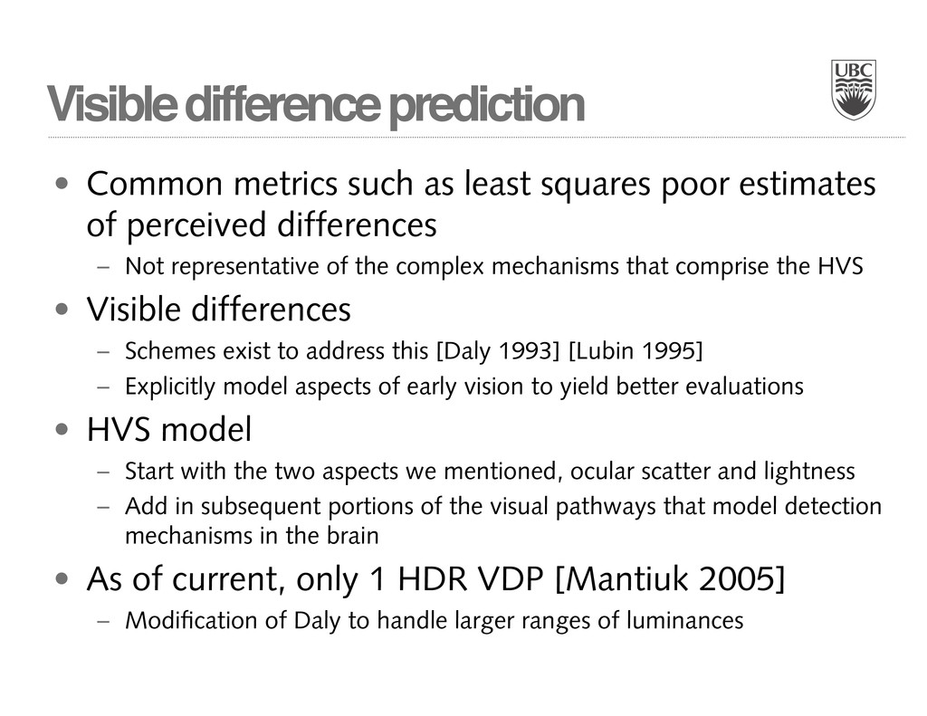
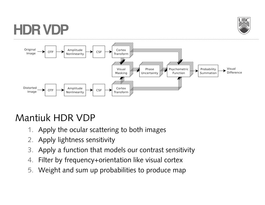
43. Evaluation • We make use of [Mantiuk 2005] HDR VDP to perform our comparisons • While the hardware limitations prevent reproducing the exact luminances of the original, a human observer cannot readily detect the majority of the differences • But first begin with two preliminary topics
44. Preliminaries • Fundamental claim of the hardware – Ocular scattering masks the low dynamic range of the LCD panel and its inability to completely compensate for the low-frequency backlight – LEDs produce white light, as is the color of the bloom outside the square – Camera has higher quality optics than the human eye and the scatter is small enough that the white bloom can be observed – A person looking at the square directly, however, would only see a red bloom due to the scattering in their eye – This can be observed by covering the square with and watching the adjacent bloom switch to white
45. HDR VDP interpretation • Red stripes on either side of a face represent that the edge is not accurately reproduced in the displayed image • Features outside the square indicate there is excessive backlight • Features inside the square indicate that the backlight is insufficiently bright and the LCD panel is clamping, and the angled features inside the corners mean the same and we can conclude that the backlight is low frequency
46. Algorithm evaluation • Compare the output of the HDR VDP for four images – Two test patterns – Two photographs. • Each set is presented the same way – The original images is on top – The displayed image is in the middle – The VDP probability overlay is at the bottom. Since both the original and displayed images are HDR, they are first tone mapped to 8 bits using Reinhard et al's photographic tone mapping operator
47. Test pattern • Combination several features – In the center are vertical and horizontal frequency gratings, and horizontal white bars above and below are linear gradients – There are solid rectangles on the left and the outlined boxes on the right are which can be used to check alignment of the display – The black level is set to 1c d/m2 and the peak intensity is set to 2200 cd/m2 – High contrast edges and features too small to get full intensity – 1.42% of pixels had more than 75% prob. – 0.71% of pixels had more than 95% prob.
48. Frequency ramp • Alternating white and black boxes – Various widths and heights – Similar to some of the DCT basis functions used by JPEG images – Once again, the black level is set to 1cd/m2 and the peak intensity is set to 2200 cd/m2 – The number of visible differences in the upper right is due to the relation between the feature shape and the LED grid – The packing of the LED grid is aligned horizontally, so while thin horizontal features can be accurately depicted, thin vertical features will cause a saw-tooth like vertical pattern that is detected – 1.15% of pixels had more than a 75% prob. – 0.79% of pixels had more than a 95% prob.
49. Apartment • First of photographs of real scenes – Depicts an indoor scene – The values are roughly calibrated to absolute photometric units, and the minimum value is 0 cd/m2 and the maximum value is 1620 cd/m2 – Compared to the test patterns, it has noticeably less error – Most natural images do not contain quite as drastic contrast boundaries as the test patterns – 0.26% of pixels had more than a 75% prob. – 0.16% of pixels had more than a 95% prob.
50. Moraine • Sample of an outdoor scene – Again, the values are roughly calibrated to absolute photometric units – Minimum value is 0 cd/m2 and the maximum value is 2200 cd/m2. – An example of an image that is perfectly represented on the display – Validates that there is nothing intrinsic in the display hardware that prevents producing artifact-free images – 0.0% of pixels had more than a 75% prob.
51. Discussion • The probabilities assigned by the VDP are based on our affect our ability to detect differences in a direct comparison • Without the original image to compare against, the user must rely on other less accurate mechanisms of determining whether a feature indicates a difference – For many applications, the user will not be comparing the display any ground truth and we can expect that detection probabilities will decrease in many areas – As long as the difference does not look out of place or wrong, the displayed image will appear as valid as the original
52. Future work • Possible areas include – Color, motion, and dependency on spatial frequency • Addressing the issue of remapping images with pixel values outside the displayable space of the monitor – Opportunity to improve and test tone mapping techniques from very high dynamic range images to HDR images that the monitor supports • Challenges inherent in the combination of LCD and variable backlight – Due to the achromatic light leaking through blacks, the darker the color, the less saturated that color is – In LDR display calibration, because the poor sensitivity of the HVS to saturation differences for lower luminances, this characteristic is approximated as a constant to be subtracted from all channels – This is not the case with the variable backlight of the HDR displays
53. Conclusions • Presented image processing algorithms for the display hardware – Approximate solutions which operate within time constraints – While still able to achieve high quality results • Validated the results using a perceptually-based objective – Highly encouraging results on normal scenes – Operates as well as possible by hardware in pathological cases • Also tested actively in commercial settings – The primary means of generating both real-time and offline content for display produce BrightSide Technologies over the last year