Defocus Techniques for Camera Dynamic Range Expansion

Slides from my Electronic Imaging 2010 talk.

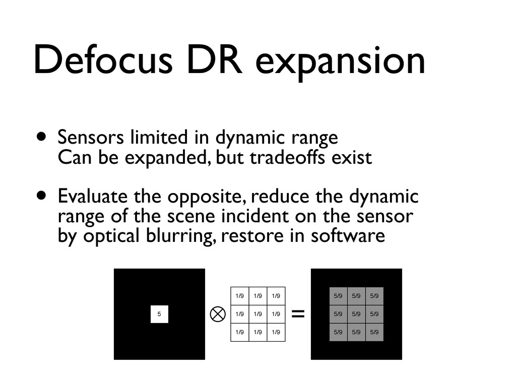
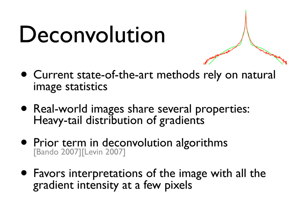
Defocus imaging techniques, involving the capture and reconstruction of purposely out-of-focus images, have recently become feasible due to advances in deconvolution methods. This paper evaluates the feasibility of defocus imaging as a means of increasing the effective dynamic range of conventional image sensors. Blurring operations spread the energy of each pixel over the surrounding neighborhood; bright regions transfer energy to nearby dark regions, reducing dynamic range. However, there is a trade-off between image quality and dynamic range inherent in all conventional sensors.

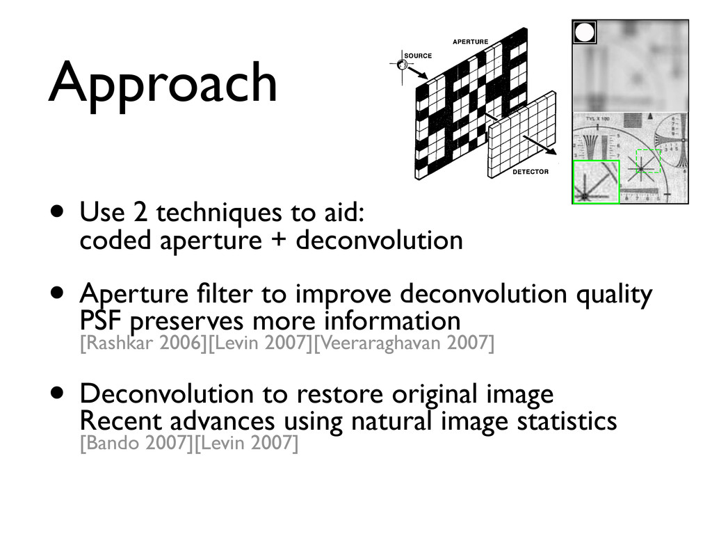
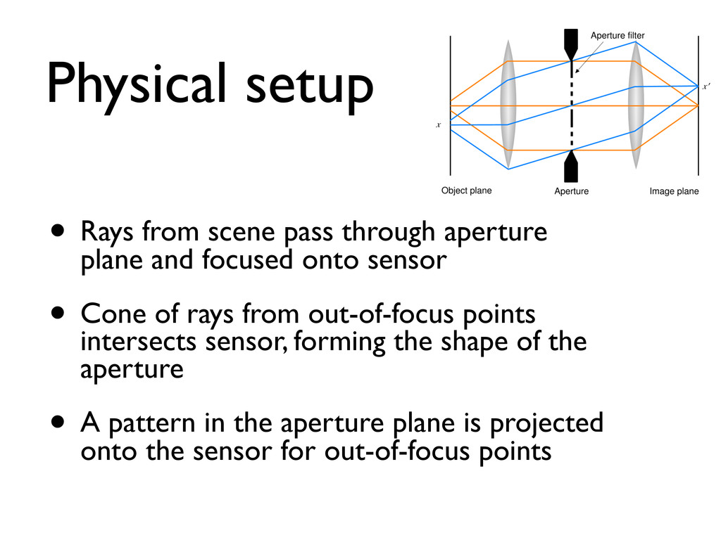
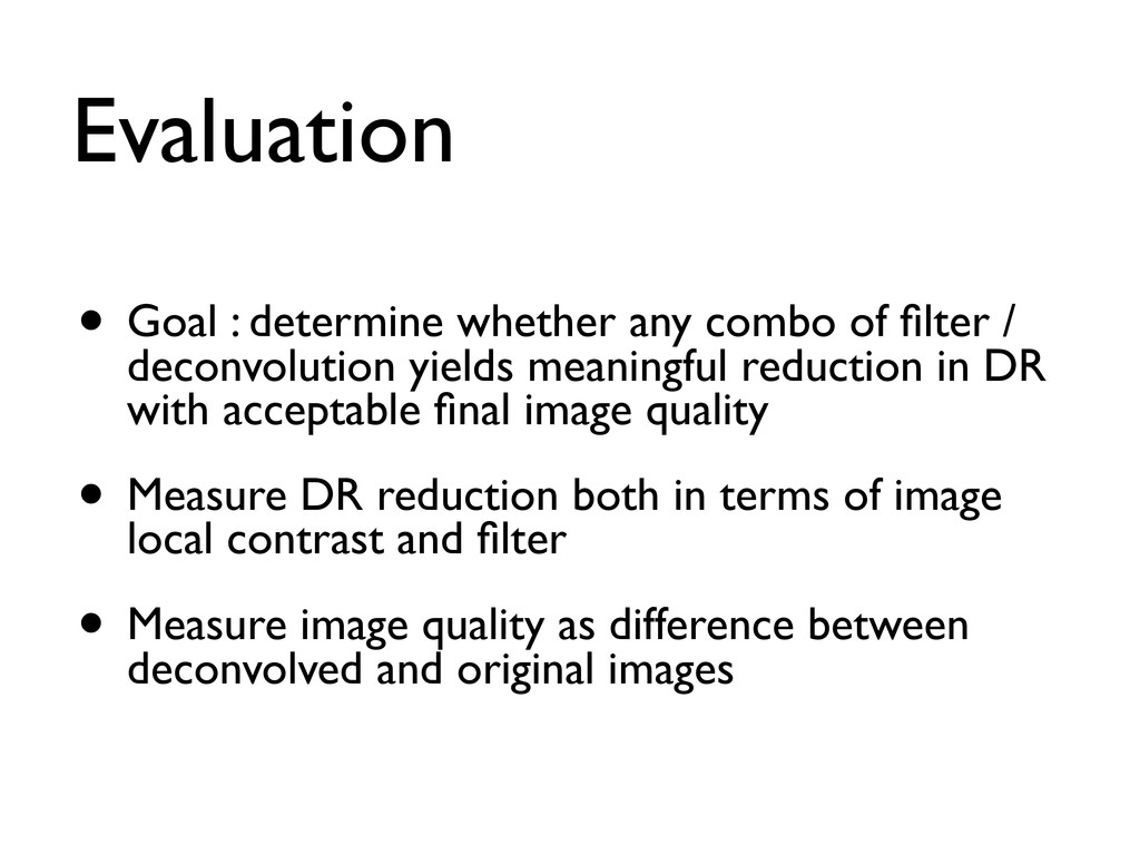
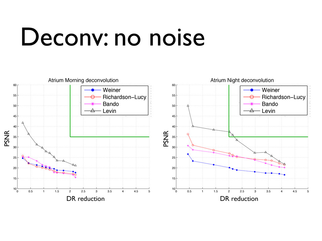
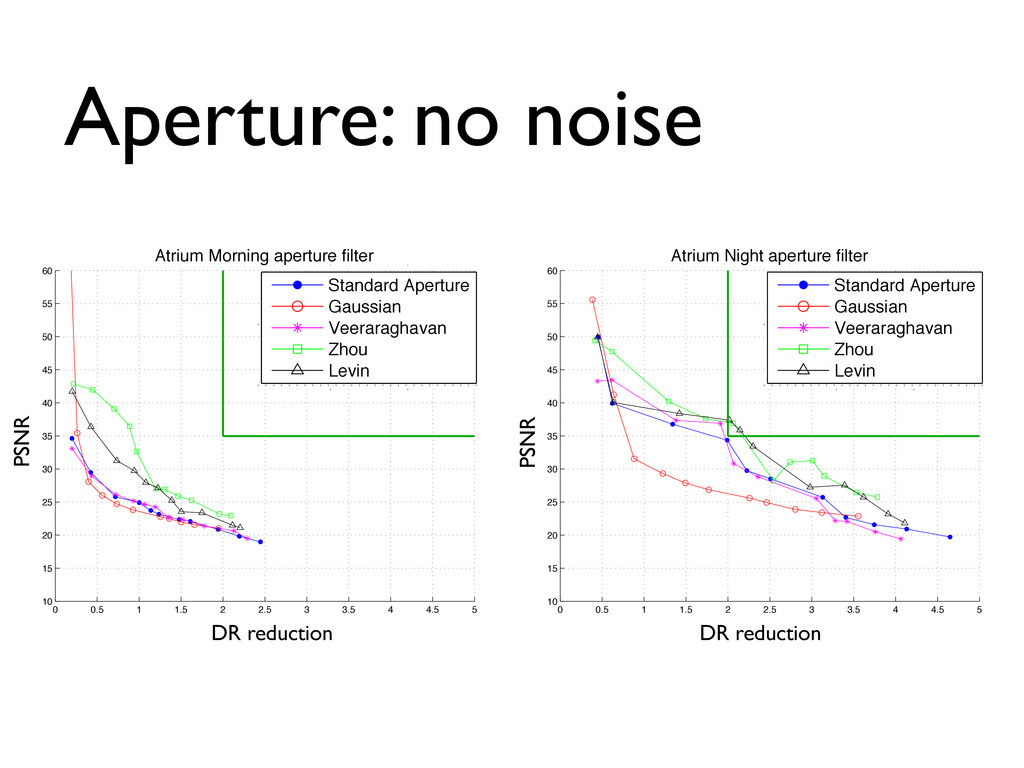
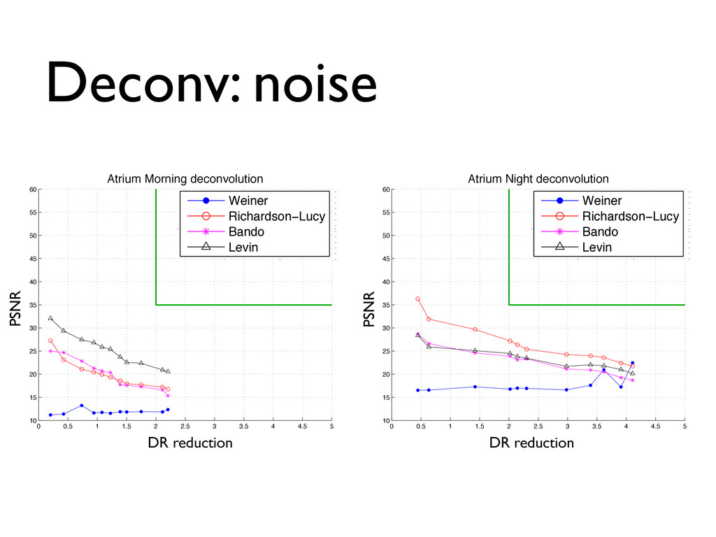
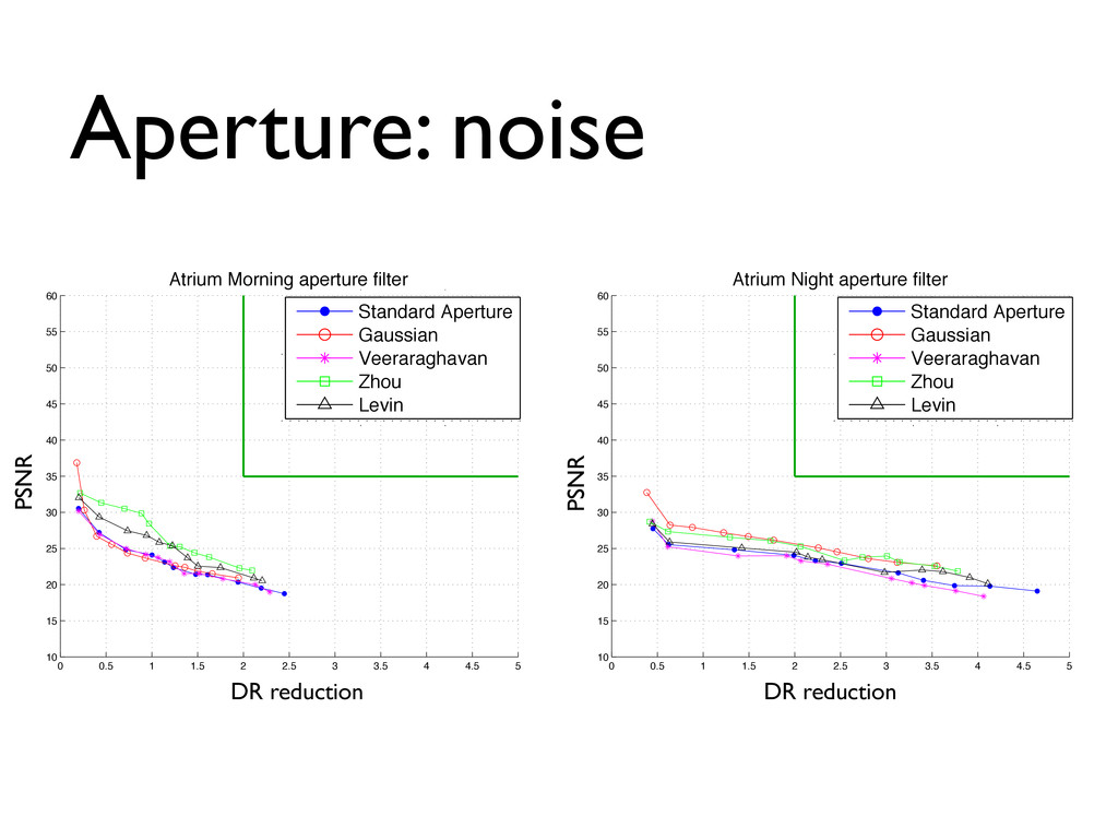
The approach involves optically blurring the captured image by turning the lens out of focus, modifying that blurred image with a filter inserted into the optical path, then recovering the desired image by deconvolution. We analyze the properties of the setup to determine whether any combination can produce a dynamic range reduction with acceptable image quality. Our analysis considers both properties of the filter to measure local contrast reduction, as well as the distribution of image intensity at different scales as a measure of global contrast reduction. Our results show that while combining state-of-the-art aperture filters and deconvolution methods can reduce the dynamic range of the defocused image, providing higher image quality than previous methods, rarely does the loss in image fidelity justify the improvements in dynamic range.

Transcript

1. Defocus Techniques for Camera Dynamic Range Expansion Matthew Trentacoste, Cheryl Lau, Mushfiqur Rouf, Rafal Mantiuk, Wolfgang Heidrich University of British Columbia
2. Defocus DR expansion • Sensors limited in dynamic range Can be expanded, but tradeoffs exist • Evaluate the opposite, reduce the dynamic range of the scene incident on the sensor by optical blurring, restore in software 5 5/9 5/9 5/9 5/9 5/9 5/9 5/9 5/9 5/9 1/9 1/9 1/9 1/9 1/9 1/9 1/9 1/9 1/9 =
3. Approach • Use 2 techniques to aid: coded aperture + deconvolution • Aperture filter to improve deconvolution quality PSF preserves more information [Rashkar 2006][Levin 2007][Veeraraghavan 2007] • Deconvolution to restore original image Recent advances using natural image statistics [Bando 2007][Levin 2007]
4. Physical setup • Rays from scene pass through aperture plane and focused onto sensor • Cone of rays from out-of-focus points intersects sensor, forming the shape of the aperture • A pattern in the aperture plane is projected onto the sensor for out-of-focus points
5. Coded Aperture • Originally from x-ray astronomy [Fenimore 1978][Gottesman 1989] • Structured arrays + decoding algorithm with resolution of pinhole, but better SNR • Employed in visible light photography [Rashkar 2006][Levin 2007][Veeraraghavan 2007] • Improve frequency properties of filter
6. Aperture filters • What makes a good filter? • Frequency response • Position and spacing of zero frequencies • Diffraction / transmission
7. Deconvolution • Restore image distorted by PSF [Wiener 1964][Richardson 1972][Lucy 1974] • Ill-posed, infinite solutions • No exact solution due to noise • Division in FFT, issues with small values in OTF of filter f = f0 ⊗ k + η
8. Deconvolution • Current state-of-the-art methods rely on natural image statistics • Real-world images share several properties: Heavy-tail distribution of gradients • Prior term in deconvolution algorithms [Bando 2007][Levin 2007] • Favors interpretations of the image with all the gradient intensity at a few pixels
9. Evaluation • Goal : determine whether any combo of filter / deconvolution yields meaningful reduction in DR with acceptable final image quality • Measure DR reduction both in terms of image local contrast and filter • Measure image quality as difference between deconvolved and original images
10. Source material Atrium Morning Atrium Night Figure 3.3: Sample images used in evaluation. Radius Atrium Morning Atrium Night min max reduction min max reduction Original 0.00 11.0 0.00 12.0 1 0.00 10.8 0.200 0.452 12.0 0.452 2 0.00 10.6 0.424 0.622 12.0 0.622 3 0.00 10.3 0.716 1.163 11.8 1.34 4 0.02 10.0 1.00 1.436 11.4 1.99 5 0.08 9.94 1.14 1.589 11.4 2.23 6 0.15 9.92 1.24 1.731 11.2 2.51 8 0.31 9.83 1.48 1.890 10.8 3.13 9 0.40 9.79 1.61 1.950 10.5 3.41 11 0.66 9.71 1.94 2.08 10.3 3.74 13 0.86 9.67 2.19 2.18 10.1 4.13 16 1.04 9.59 2.45 2.26 9.61 4.65 Figure 3.4: Amount of reduction in dynamic range as a function of radius of a standard aperture (disk) filter in pixels. All units are in terms of powers of two, referred to as exposure value (EV) stops. Atrium Morning Atrium Night
11. Source material Atrium Morning Atrium Night Figure 3.3: Sample images used in evaluation. Radius Atrium Morning Atrium Night min max reduction min max reduction Original 0.00 11.0 0.00 12.0 1 0.00 10.8 0.200 0.452 12.0 0.452 2 0.00 10.6 0.424 0.622 12.0 0.622 3 0.00 10.3 0.716 1.163 11.8 1.34 4 0.02 10.0 1.00 1.436 11.4 1.99 5 0.08 9.94 1.14 1.589 11.4 2.23 6 0.15 9.92 1.24 1.731 11.2 2.51 8 0.31 9.83 1.48 1.890 10.8 3.13 9 0.40 9.79 1.61 1.950 10.5 3.41 11 0.66 9.71 1.94 2.08 10.3 3.74 13 0.86 9.67 2.19 2.18 10.1 4.13 16 1.04 9.59 2.45 2.26 9.61 4.65 Figure 3.4: Amount of reduction in dynamic range as a function of radius of a standard aperture (disk) filter in pixels. All units are in terms of powers of two, referred to as exposure value (EV) stops. Atrium Morning Atrium Night 2.45 EV
12. Source material Atrium Morning Atrium Night Figure 3.3: Sample images used in evaluation. Radius Atrium Morning Atrium Night min max reduction min max reduction Original 0.00 11.0 0.00 12.0 1 0.00 10.8 0.200 0.452 12.0 0.452 2 0.00 10.6 0.424 0.622 12.0 0.622 3 0.00 10.3 0.716 1.163 11.8 1.34 4 0.02 10.0 1.00 1.436 11.4 1.99 5 0.08 9.94 1.14 1.589 11.4 2.23 6 0.15 9.92 1.24 1.731 11.2 2.51 8 0.31 9.83 1.48 1.890 10.8 3.13 9 0.40 9.79 1.61 1.950 10.5 3.41 11 0.66 9.71 1.94 2.08 10.3 3.74 13 0.86 9.67 2.19 2.18 10.1 4.13 16 1.04 9.59 2.45 2.26 9.61 4.65 Figure 3.4: Amount of reduction in dynamic range as a function of radius of a standard aperture (disk) filter in pixels. All units are in terms of powers of two, referred to as exposure value (EV) stops. Atrium Morning Atrium Night 2.45 EV 4.56 EV
13. Tests • Filters evaluated: • Normal aperture • Gaussian • Veeraraghavan • Levin • Zhou • Deconvolution evaluated: • Wiener filtering • Richardson-Lucy • Bando • Levin
14. Evaluation (cont) • Success criteria: • Reduction of at least 2 stops to justify the computational cost of deconv • Quality of at least PSNR 35
15. Images Weiner Richardson-Lucy Bando Levin filter=Zhou, noise = 0, radius = 1
16. Images Weiner Richardson-Lucy Bando Levin filter=Zhou, noise = 0, radius = 5
17. Images Weiner Richardson-Lucy Bando Levin filter=Zhou, noise = 0, radius = 16
18. Deconv: no noise 0 0.5 1 1.5 2 2.5 3 3.5 4 4.5 5 10 15 20 25 30 35 40 45 50 55 60 Dynamic range reduction (EV stops) PSNR (dB) Atrium Morning deconvolution Weiner Richardson−Lucy Bando Levin 0 0.5 1 1.5 2 2.5 3 3.5 4 4.5 5 10 15 20 25 30 35 40 45 50 55 60 Dynamic range reduction (EV stops) PSNR (dB) Atrium Night deconvolution Weiner Richardson−Lucy Bando Levin DR reduction DR reduction PSNR PSNR orning deconvolution Weiner Richardson−Lucy Bando Levin 25 30 35 40 45 50 55 60 PSNR (dB) Atrium Morning deconvolution Weiner Richardson−Lucy Bando Levin
19. Aperture: no noise 0 0.5 1 1.5 2 2.5 3 3.5 4 4.5 5 10 15 20 25 30 35 40 45 50 55 60 Dynamic range reduction (EV stops) PSNR (dB) Atrium Morning aperture filter Standard Aperture Gaussian Veeraraghavan Zhou Levin 0 0.5 1 1.5 2 2.5 3 3.5 4 4.5 5 10 15 20 25 30 35 40 45 50 55 60 Dynamic range reduction (EV stops) PSNR (dB) Atrium Night aperture filter Standard Aperture Gaussian Veeraraghavan Zhou Levin DR reduction DR reduction PSNR PSNR Morning aperture filter Standard Aperture Gaussian Veeraraghavan Zhou Levin 20 25 30 35 40 45 50 55 60 PSNR (dB) Atrium Morning aperture filter Standard Aperture Gaussian Veeraraghavan Zhou Levin
20. Deconv: noise 0 0.5 1 1.5 2 2.5 3 3.5 4 4.5 5 10 15 20 25 30 35 40 45 50 55 60 Dynamic range reduction (EV stops) PSNR (dB) Atrium Morning deconvolution Weiner Richardson−Lucy Bando Levin 0 0.5 1 1.5 2 2.5 3 3.5 4 4.5 5 10 15 20 25 30 35 40 45 50 55 60 Dynamic range reduction (EV stops) PSNR (dB) Atrium Night deconvolution Weiner Richardson−Lucy Bando Levin DR reduction DR reduction PSNR PSNR orning deconvolution Weiner Richardson−Lucy Bando Levin 25 30 35 40 45 50 55 60 PSNR (dB) Atrium Morning deconvolution Weiner Richardson−Lucy Bando Levin
21. Aperture: noise 0 0.5 1 1.5 2 2.5 3 3.5 4 4.5 5 10 15 20 25 30 35 40 45 50 55 60 Dynamic range reduction (EV stops) PSNR (dB) Atrium Morning aperture filter Standard Aperture Gaussian Veeraraghavan Zhou Levin 0 0.5 1 1.5 2 2.5 3 3.5 4 4.5 5 10 15 20 25 30 35 40 45 50 55 60 Dynamic range reduction (EV stops) PSNR (dB) Atrium Night aperture filter Standard Aperture Gaussian Veeraraghavan Zhou Levin DR reduction DR reduction PSNR PSNR Morning aperture filter Standard Aperture Gaussian Veeraraghavan Zhou Levin 20 25 30 35 40 45 50 55 60 PSNR (dB) Atrium Morning aperture filter Standard Aperture Gaussian Veeraraghavan Zhou Levin
22. Conclusions • Levin deconv the best, obtaining results with coded filters at very low noise levels • No combination of filter and deconvolution consistently produced acceptable results • Efficiency of the approach is scene dependent Most efficient for small, isolated bright regions