Upgrade to PRO for Only $50/Year—Limited-Time Offer! 🔥

The Fusion of Mathematical Optimization and AI ...

Avatar for MIKIO KUBO MIKIO KUBO
December 04, 2025

The Fusion of Mathematical Optimization and AI (MOAI): History and Outlook (Final Version)

The Fusion of Mathematical Optimization and AI (MOAI): History and Outlook

Avatar for MIKIO KUBO

MIKIO KUBO

December 04, 2025
Tweet

More Decks by MIKIO KUBO

Other Decks in Research

Transcript

  1. Self-introduction https://www.youtube.com/@kubomikio https://x.com/MickeyKubo https://www.logopt.com/kubomikio/ Tokyo University of Marine Science and

    Technology: Professor Moai Lab : Director & CTO A-Star Quantum: Director Optimind: Advisor Ridge-i: Technical Advisor
  2. Mathematical Optimization (MO) + Artificial Intelligence (AI) Real Problem MO

    Optimizaiton AI Machine Learning Metaheuristics Constraint Programming
  3. MOAI = Fusion of Three Fields Mathematical Optimization Metaheuristics Machine

    Learning Deep Learning LLMs, Gen. AI, Agentic AI MOAI Hierarchical building block AutoOpt Math-heuristics Distributionally robust optimization Encode-decode method MO hybrid for dynamic stochastic models End-to-end learning Supply chain modeling language Modeling and app generation with agentic AI (AGI4OPT) Automatic decomposition Instance similarity
  4. History of Mathematical Optimization 1947 Dantzig Simplex method 1984 Karmarker

    Interior point method 1971 Cook’s Theorem NP-completeness 1957 Bellman Dynamic programming 1958 Gomory Cutting plane 1945 Stigler’s Diet Problem First linear program 1989 Kojima Primal-dual interior point method 1954 Dantzig-Fulkerson-Johnson Traveling salesman problem 1979 Khachiyan Ellipsoid method 2008- Gurobi 1988- CPLEX 1985 AMPL A Math. Prog. Language
  5. History of Metaheutristics 1983 Kirkpatrick et al. Simulated annealing 1975

    Holland Genetic algorithm 1953 Metropolis et al. Markov chain Monte Carlo 1986 Glover Tabu search 1989-1990s Johnson et al. Experimental analsis 1977 Glover Scatter search 1970 & 73 Keinighan-Lin Variable depth local search 1995 Wolpert-Macready No free lunch theorem 2001 Kubo-Miyamoto Hierarchical building block method 2002 Nonobe-Ibaraki RCPSP solver
  6. 2012 AlexNet History of Deep Learning and Neural Net (NN)

    1943 McCulloch-Pitts Perceptron 1987 LeCun Convolutional NN 1979 Fukushima Neocognitoron 2015 ResNet 2017 Transformer 2018 GPT 1958 Resenblatt Perceptron machine 1997 Hochreiter–Schmidhuber LSTM 1985 Hinton et al. Backpropagation 2006- Fei-Fei Li ImageNet 2014 Goodfellow GAN 1982 Hopfield Hopfield machine 1972 Amari Recurrent NN 1969 Fukushima ReLU 1967 Amari Multilayer perceptoron 2021 Stable Diffusion 2022 ChatGPT 2015 Tensorflow
  7. Abbreviations and classification • MO:Mathematical Optimization • O:Optimization • ML:

    Machine Learning • RL:Reinforcement Learning = O + ML • MPC:Model Predictive Control = O + ML Fusion of MO and ML  Categorized into 7 patterns 1. ML -> MO (ML-first MO-second) 2. MO -> ML (MO-first ML-second) 3. MO ⊃ ML (ML assists MO, ML4MO) 4. ML ⊃ MO(MO assists ML, MO4ML) 5. Mutual Engagement with Basic Optimization Theory 6. ML & MO assists RL/MPC 7. LLMs (ChatGPT , Claude, Gemini) assist “modeling” of MO
  8. Conceptual diagram of fusion patterns ML MO ML -> MO

    (ML-first MO-second) MO -> ML (MO-first ML-second) ML MO MO ⊃ ML (ML assists MO, ML4MO) ML ⊃ MO(MO assists ML, MO4ML) Mutual Engagement with Basic Optimization Theory RL/MPC MO ML MO ML ML MO ML MO RL/MPC LLM assists MODELING ML MO MODELING LLM
  9. Pattern1 ML → MO Apply MO after making predictions in

    ML The most classic and natural (predict and then optimize) approach 1. Predict with ML and function approximation = > Solve the approximate constraint or objective function with MO ✓ Embedding ML prediction models as mathematical formulas in MO (Gurobi 10.0+) ✓ Optimize ML as a black box ✓ Approximate an ML prediction model as an MO-solvable function with realistic assumptions 2. Preprocessing with ML (e.g., clustering) → MO ML MO Data Solution
  10. ML -> MO (Constraint Learning) • Gurobi ML https://github.com/Gurobi/gurobi-machinelearning •

    Linear regression • Polynomial regression (quadratic) • Logistic regression (approximating nonlinear functions with piecewise linear functions) • Neural network (fully connected layer and LeLU only) • decision tree • Gradient Boosting • Random Forest ML y x Feature vector (variable or constant) Forecast constraints target min f(x,y) s.t. x => ML => y x ∈X
  11. Any ML-> Black BoxO • Black-box optimization with ML as

    an oracle • Advantage: Runs on any ML • Weaknesses: Slow ML f(x) x min f(x) s.t. x ∈X Black-Box Optimization x f(x) oracle
  12. ML -> Approximate easy-to-solve functions -> solver • Generate supervised

    data with any ML model • Assume easy-to-solve functions and approximate functions to satisfy practical axioms • Example 1: Transportation costs between points and by mode of transport Monotonic non-reduction (heavier and higher or the same) Continuous (does not change suddenly) Concave function (the cost per unit weight decreases as the weight increases) Go through the origin (free if you don't carry it) • Example 2: Demand Function Decreasing and convex functions for price • => Piecewise linear regression with MO
  13. Pre-processing with ML → MO • Unsupervised ML, such as

    clustering and dimensionality reduction, is a kind of optimization • For large-scale optimization, preprocessing is natural • Examples of Logistics Network Design Problems • Cluster 1000 points to 50 points and then optimize
  14. Contextual Stochastic Optimization (1) • Predict-then-Optimize • Linear optimization (variable

    x , cost vector c) • Context F and contextual and cost training data {F,c} • Conditional probability distribution of c under context F 𝐷𝐹 Compute Ƹ 𝑐 = 𝑐 𝐹 ] (e.g., using least squares),then minimize Ƹ 𝑐𝑇x min 𝑥∈𝑋 𝐸𝑐∈𝐷𝐹 𝑐𝑇𝑥 𝐹 ] = min 𝑥∈𝑋 𝐸𝑐∈𝐷𝐹 𝑐 𝐹 ]𝑇 𝑥 Predicted value ML Least square (M)O Linear Optimization Data Solution F c
  15. Contextual Stochastic Optimization (2) Loss function for the difference from

    the case of optimization based on the realized value of the cost (Smart Predict-then-Optimize/Decision-Focused Learning) Optimal solution oracle The optimal value when the realized value is known 𝑧∗ 𝑐 = min 𝑥∈𝑋 𝑐𝑇𝑥 𝐿𝑂𝑆𝑆+ Ƹ 𝑐, 𝑐 = max { 𝑥∈𝑋 𝑐𝑇𝑥 − 2 Ƹ 𝑐𝑇𝑥 } + 2 Ƹ 𝑐𝑇𝑥∗ 𝑐 − 𝑧∗ 𝑐 𝐿𝑂𝑆𝑆 Ƹ 𝑐, 𝑐 = 𝑐𝑇𝑥∗ ෝ 𝑐 − 𝑧∗ 𝑐 SPO loss(non-convex) SPO+ loss(convex) 𝑥∗ Upper bound of SPO loss (M)O Linear Optimization Data Solution ML SPO+ loss min. F Prediction Realization
  16. Decision-Focused Learning Software PyEPO https://github.com/khalil-research/PyEPO ✓ SPO+ Smart Predict-then-Optimize ✓

    DBB Differentiable Black-box Optimizer ✓ DPO Differentiable Perturbation Optimizer ✓ PYFL Pertubated Fenchel-Young Optimizer ✓ NCE Noise Contrastive Estimation ✓ LTR Learning to Rank Smart “Predict, then Optimize” A. N. Elmachtoub and P. Grigas Management Science, Volume 68
  17. Estimation-then-Optimize • Scenario Generation Approach to Contextual Stochastic Optimization •

    Data (F,Y): Y is the data to be used in the optimization, F is the auxiliary (contextual) data. • F (e.g., google trend) is observable, Y (forecast) predicts demand • Create a prediction model with ML and generate a predicted value Y and a weight (probability) w from the observed F • Stochastic (weighted against scenario) optimization from Y and w Bertsimas, D. & Kallus, N. 2019 From Predictive to Prescriptive Analytics. Management Science 66(3):1025- 1044. ML Stochastic Optimization Data (Y, F) Solution Instances weight w Bertsimas, D., Kallus, N., & Hussain, A. (2016). Inventory Management in the Era of Big Data. Production and Operations Management, 25, 2006-2009. F Y
  18. Challenges of ML → MO • Simply incorporating an ML

    model into MO increases the amount of computation. • Combining a large-scale ML model with a large-scale MO model is problem-dependent • Application examples are mainly simple ones such as inventory optimization
  19. Pattern 2 MO → ML • Machine learning after optimization

    • Example: Shipping Optimization with Known Past Customer Demand • Optimization is performed on historical data to find the minimum number of trucks for each day • A regression model that predicts the number of trucks based on past day information. ML MO Data Solution
  20. Pattern 3 MO ⊃ ML, ML4MO ML assists MO (objective

    is optimization) 1. Selection of solution method, setting of (hyper) parameters of solution method, selection of algorithm in ML 2. ML/RL inside the Optimization Branching rules and excision planes are improved with ML (RL) 3. Combinatorial optimization with reinforcement learning 4. Generate data (instance and solution pair) using MO and train it with ML Use ML to speed up MO for new problem example 1. ML returns solution hints and constraints to be satisfied, speeding up MO (MIPlearn) 2. ML returns an approximate (infeasible) solution and converts it to a close feasible solution (optimization proxy) 3. ML returns equality constraints and the values of an integer variables and generates a solution from it (optimization voice)
  21. Classification of ML4MO Solution ML ML returns Solution (Using MO

    to create training data) MO Instances Solution ML Parameter Algorithm ML before optimization Instances Instances Instances MO Solution ML ML inside optimization Solution RL Solving Combinatorial Optimization Problems with RL
  22. Learning MO performance and selecting solution methods (parameters) • Learn

    the performance of multiple optimization methods and select a solution method (parameter) with a trained ML model Instances ML Optimization Methods Time vs Solution Rewards Pre-trained ML መ 𝑓(𝑎) Learning the performance of various optimization methods Instances Optimization ML → MO MO → ML Solution Methos Parameters Solution Selecting methods or parameters with pre-trained ML models
  23. Acceralation of MIP • Solving Mixed Integer Programs Using Neural

    Networks (Deep Mind, Google Research) • Apply to general MIP (Mixed Integer Programming) using Graph Neural Net
  24. Solving Combinatorial Optimizatio using RL • TorchRL (PyTorch) based library

    RL4CO • Attention Model + Proximity Policy Optimization (Reinforcement Learning) • Experimented with small and medium-sized TSPs (and their variants) (performance is a little better than greedy) • Addresses scheduling issues (incomplete) • Other similar studies have focused on small- to medium-scale experiments • The challenge is whether it can be scaled to large-scale problem examples.
  25. MIPLearn Instances MO Prefiction ML 𝐼(𝑖) (𝑖 = 1, …

    , 𝑚) 𝑂𝑃𝑇 𝐼 Optimal Solution 𝑋(𝑖) (𝑖 = 1, … , 𝑚) Instances Solutions Training Data New Instance Distribution of Optimal Solutions 𝐼 x.Start (Starting Solution) x.VarHintVal(Variable Hint) Additional constrraints that must be satisfied
  26. Applictions of MIPlearn • Using the unit commitment problem as

    an example to accelerate mathematical optimization with machine learning • Fixing variables from training data with k-nearest neighbors and SVMs • Packages for general optimization problems https://anl-ceeesa.github.io/MIPLearn/ • Application to TSP and knapsack problems (only the numerical information changes) Álinson S. Xavier, Feng Qiu, Shabbir Ahmed (2020) Learning to Solve Large-Scale Security-Constrained Unit Commitment Problems. INFORMS Journal on Computing 33(2):739-756
  27. Optimization Proxies • Application to Optimization of Power Transmission Flow

    Problem (End-to-end learning and repair) • Lagrange relaxation to meet constraints End-to-End Feasible Optimization Proxies for Large-Scale Economic Dispatch Wenbo Chen, Mathieu Tanneau, Pascal Van Hentenryck Proxies
  28. Optimization Voice • Learn strategies (inequality constraints that become equal

    signs and values of integer variables) with optimal decision trees and NNs • Assume that the parameters of the example problem vary within a narrow range • Fast solution to new problem examples • Package https://github.com/bstellato/mlopt Examples of inventory optimization and knapsacks Bertsimas-Stellaato (2019) “Online Mixed-integer optimization in millseconds”
  29. Optimization Voice 朱制約 朱 Integer Var.s Constraints (Inequality Constraints) 朱

    Continuous Var.s 朱 Equalities in opt. sol.s 朱 朱 Values of Integer Var.s Optimization Voice (Strategy) Online Optimization (Instances of mixed-integer optimization problems with slightly varying parameters Learn the integer variables and the constraints that become equalities in the training phase For a new instance, multiple strategies are predicted The best solution among them is then selected Solve the system of linear equations
  30. MIPLearn, Optimization Proxies and Voice ML Instances MIPLearn MO Solution

    Solution Hint Optimization Proxies Repair Layers Solution Infeasible Solution (Proxiy) ML Solution Integer Var.s Equality Constraints Optimization Voice Deep Learning The problem structure remains constant while only the numerical values change + Lagrange Relaxation Motivation: directly learning feasible solutions through machine learning is difficult Solve the system of linear equations
  31. Encode-Decode Method ML Instances Decoder Solution An Encoding of Solution

    Example: Scheduling Problem Priority of jobs + mode of jobs: Decoding is an active schedule generation scheme Priority of jobs: Decoding is optimized using a scheduling solver, OptSeq Example: Delivery Planning Problem Pre-cycle (decoding is dynamic programming) Assignment to vehicles (with overlap for flexibility) + pre-cycle circuits (decoding is a recourse strategy) An algorithm to quickly recover the solution based on the encoding Encoding Decoder MIPlearn Additional Constraints MIP Solver Opt. Proxies Infeasible Sol.s Repair Layers Opt. Voice Equality Constraints Values of Integer Var.s System of Linear Equations Complexity of Encoding << Complexity of Solution
  32. Challenges of ML4MO • The training and test examples need

    to be "close" • Useful when the structure of the instances is the same but the numerical value is different. • It is necessary to define ”similarity" of problem instances with different structures. • In many numerical experiments, "similar" problem instances are artificially generated and evaluated. • There are few cases for real-world problems (with the exception of electric power applications)
  33. Pattern 4 ML ⊃ MO, MO4ML • Perform ML tasks

    (classification, regression) using (M)O • MO model for feature selection and MO model for optimal decision tree • Application of Optimization Methods for Constrained ML Models (e.g., Lagrange Relaxation) MO Data Classification Regression ML MO assists ML (the main objective is machine learning)
  34. Construct Decision Trees using Optimization Survey paper Carrizosa, E., Molero-Río,

    C. & Romero Morales, D. Mathematical optimization in classification and regression trees. TOP 29, 5–33 (2021) • Classical CART (Greedy) • Probabilistic branching using continuous nonlinear optimization • Decision trees by MIP
  35. Optimal Classification Tree with MIP Bertsimas-Dunn (2017) Optimal classification trees.

    Mach. Learn. 106(7):1039–1082 • Optimal Classification Tree • High Interpretability • Extensive Computation Time For Speeding up (mainly for categorial data) ✓ Selecting data subsets ✓ formulations specific to binary classification ✓ flow formulations ✓ Benders decomposition ✓ constraint optimization ✓ approximate optimization ✓ data mining techniques ✓ dynamic programming
  36. Open-source Packages for Optimal Decision Trees • https://github.com/LucasBoTang/Optimal_Classification_Trees Comparison of

    OCT (Optimal Classification Tree), BinaryOCT, flowOCT • MurTree https://bitbucket.org/EmirD/murtree/src/master/ Dynamic Programming • DL8.5 https://dl85.readthedocs.io/en/latest/user_guide.html Branch and Bound using Data Mining • https://github.com/pan5431333/pyoptree OCT and Local Search
  37. Smmary of MO4ML • Applying mathematical optimization techniques to machine

    learning is a powerful tool when used correctly • Several fast methods have been proposed for categorical data • For continuous data, it is necessary to either apply appropriate discretization or use approximate optimization
  38. Pattern 5 Cross-pollination at the Foundational Level • Optimization aspect

    shares the same fundamental ✓ Optimization in DL(Nonconvex nonlinear optimization) Momentum, Adam, fit-one cycle (experimental) ✓ Nondifferential optimization theory Nesterov acceleration Theoretical convergence proofs • Mathematical optimization is used to interpret machine learning models mathematically ✓ Insight for improvements (add sparcity to models) ✓ Convergence proofs ✓ New model ideas
  39. Pattern 6 Fusion of Dynamic Models • Dynamic optimization problems

    where future information is either unavailable or uncertain • Blending the following disciplines: ✓ Dynamic Programming (DP),Approximate DP ,neuro DP ✓ Reinforcement Learning (RL) ✓ Model Predictive Control (MPC) ✓ Multi-period stochastic or robust optimization with affine recourse function adjustment inspired by linear feedback in control MO Instances Solution ML RL/MPC
  40. MPC (Model Predictive Control) • Model Predictive Control = Prediction

    (ML) + Optimization (O) • Similar to the rolling horizon method • Controlled by repeating the optimization solution for a finite period of time • Forecasts are updated every time. • Objective function for smooth control and state stability (convex quadratic optimization) https://en.wikipedia.org/wiki/Model_predictive_control
  41. Approximate Dynamic Programming (ADP) • Approximate Dynamic Programming: Solving the

    Curses of Dimensionality (Wiley) W. B. Powell • A series of studies on approximate dynamic programming. • Fusion of DP (RL) and mathematical optimization • Application to long-distance transportation problems
  42. State After the Action State Action Post-action State Next State

    𝑠𝑡 𝑎𝑡 𝑠′𝑡 𝑠𝑡+1 Random factor 𝜖𝑡 State Action Next State 𝑠𝑡 𝑎𝑡 𝑠𝑡+1 Random factor 𝜖𝑡 Normal Dynamic Planning (DP): the number of states or actions × the state is enormous Approximate Dynamic Design (ADP): the number of post-action states is small: approximation by extracting only the features of the states
  43. Comparison of DP/RL/MPC/Stochastic (Robust) / MO Hybrid DP Approx. DP

    RL MPC Stochastic (Robust) Optimization MO Hybrid Model ◯ ◯ △ ◯ ◯ ◯ Forecasting ◯ ◯ Forecast using past instances and contexts Value Function ◯ ◯ (Post-Action State) ◯ ◯ Define on states and post-action states Optimization Greedy One-period Optimization Greedy Tree Search, Beam Search, Rollout Finite Horizon (Convex Quadratic Optimization) Stochastic (Robust) Optimization (M)O on a finite horizon problem using here and now and recourse variables + ML Approximate Value Function Piecewise Linear Functions Deep Learning Pircewise-linear, Neural Net, Decision Tree Adjustable Function ◯ ◯ ◯
  44. MO Hybrid = ML+(M)O+MPC+RL (M)O Forecast Instance Generation Solution Training

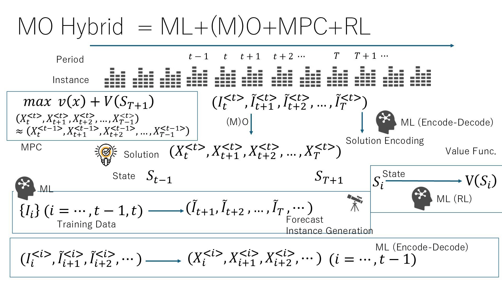
    Data Period Instance 𝑡 − 1 𝑡 𝑡 + 1 𝑡 + 2 ⋯ 𝑇 𝑇 + 1 ⋯ (𝐼𝑡 <𝑡>, ሚ 𝐼𝑡+1 <𝑡>, ሚ 𝐼𝑡+2 <𝑡>, … , ሚ 𝐼𝑇 <𝑡>) (𝑋𝑡 <𝑡>, 𝑋𝑡+1 <𝑡>, 𝑋𝑡+2 <𝑡>, … , 𝑋𝑇 <𝑡>) (ሚ 𝐼𝑡+1 , ሚ 𝐼𝑡+2 , … , ሚ 𝐼𝑇 , ⋯ ) ML ML (Encode-Decode) ML (Encode-Decode) State 𝐼𝑖 (𝑖 = ⋯ , 𝑡 − 1, 𝑡) (𝑋𝑖 <𝑖>, 𝑋𝑖+1 <𝑖>, 𝑋𝑖+2 <𝑖>, ⋯ ) (𝑖 = ⋯ , 𝑡 − 1) (𝐼𝑖 <𝑖>, ሚ 𝐼𝑖+1 <𝑖>, ሚ 𝐼𝑖+2 <𝑖>, ⋯ ) Solution Encoding 𝑆𝑡−1 𝑆𝑖 ML (RL) V 𝑆𝑖 𝑆𝑇+1 𝑚𝑎𝑥 𝑣 𝑥 + 𝑉 𝑆𝑇+1 𝑋𝑡 <𝑡>, 𝑋𝑡+1 <𝑡>, 𝑋𝑡+2 <𝑡>, … , 𝑋𝑇−1 <𝑡> ≈ 𝑋𝑡 <𝑡−1>, 𝑋𝑡+1 <𝑡−1>, 𝑋𝑡+2 <𝑡−1>, … , 𝑋𝑇−1 <𝑡−1> MPC State Value Func.
  45. Horizontal AI vs Vertical AI Horizontal AI Vertical AI Health

    Care Legal Sector Financial Service Supply Chain Optimization Open AI GPT, Google Gemini, Anthorpic Claude Tempus, PathAI, Viz.ai, Aidoc, Abridge. … Harvey, EvenUp, Oronclad, Casetext, Everlaw, … Zest AI, HighRadius, ThetaRay, BioCatch, …
  46. AGI4OPT(Hearing=>Opt. App.) User Classification Agent SC Network Design Vehicle Routing

    Production Scheduling Inventory Policy … Hearing Agent AMPL Modeling +Coding Agent Code Execusion Agent https://www.moai-lab.jp/products/agi4opt >=10000 articles >= 50 books Optimization Agent Data Mapping/ Visualization Agent (Agentic Data Scientist) UI Generation Agent Data Upload Data Upload
  47. MOAI Data Platform Agentic IBP ERP Data Production Scheduling Lot

    Sizing Logistics/Service Network Design Vehicle Routing Supply Chain Risk Optimization Stage BOM Safety Stock Allocation Inventory Policy Optimization Shift Scheduling Data Mapping