Talk at Istituto Veneto, Venice, 14 April 2016

Talk at IUTAM Symposium "Helicity, Structures and Singularity in Fluid and Plasma Dynamics", Venice, ITALY, 11-15 April 2016

Transcript

1. Atypical late-time singular regimes accurately diagnosed in stagnation-point-type helical solutions of 3D Euler flows Principal Investigator: Miguel D. Bustamante Postdoc: Dan Lucas (SFI) PhD students: Rachel Mulungye (HEA), Brendan Murray (SFI) Complex and Adaptive Systems Laboratory School of Mathematics and Statistics University College Dublin April 14th 2016 M D Bustamante (UCD) IUTAM 2016 April 14th 2016 1 / 22
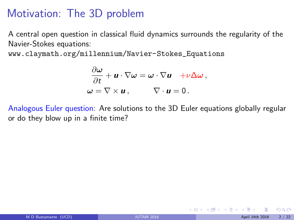
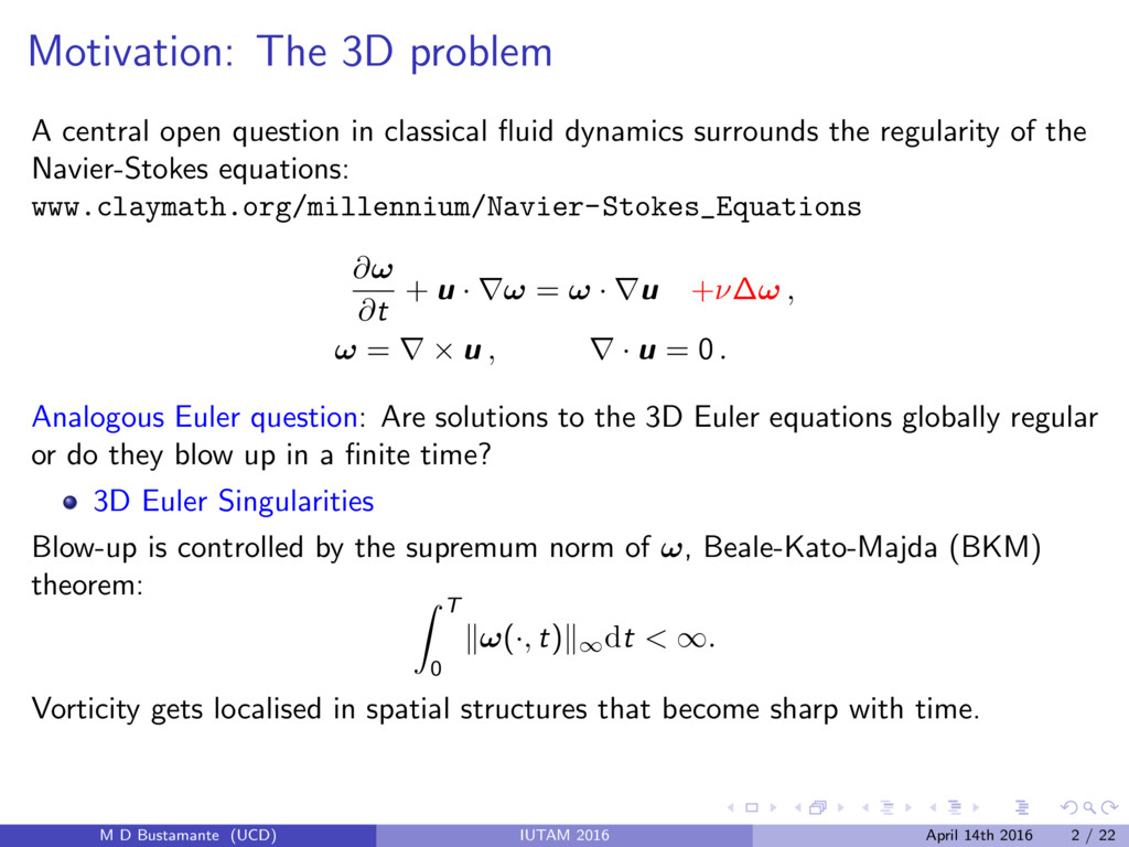
2. Motivation: The 3D problem A central open question in classical fluid dynamics surrounds the regularity of the Navier-Stokes equations: www.claymath.org/millennium/Navier-Stokes_Equations @! @t + u · r! = ! · r u +⌫ ! , ! = r ⇥ u , r · u = 0 . Analogous Euler question: Are solutions to the 3D Euler equations globally regular or do they blow up in a finite time? M D Bustamante (UCD) IUTAM 2016 April 14th 2016 2 / 22
3. Motivation: The 3D problem A central open question in classical fluid dynamics surrounds the regularity of the Navier-Stokes equations: www.claymath.org/millennium/Navier-Stokes_Equations @! @t + u · r! = ! · r u +⌫ ! , ! = r ⇥ u , r · u = 0 . Analogous Euler question: Are solutions to the 3D Euler equations globally regular or do they blow up in a finite time? 3D Euler Singularities Blow-up is controlled by the supremum norm of !, Beale-Kato-Majda (BKM) theorem: Z T 0 k!(·, t)k1dt < 1. Vorticity gets localised in spatial structures that become sharp with time. M D Bustamante (UCD) IUTAM 2016 April 14th 2016 2 / 22
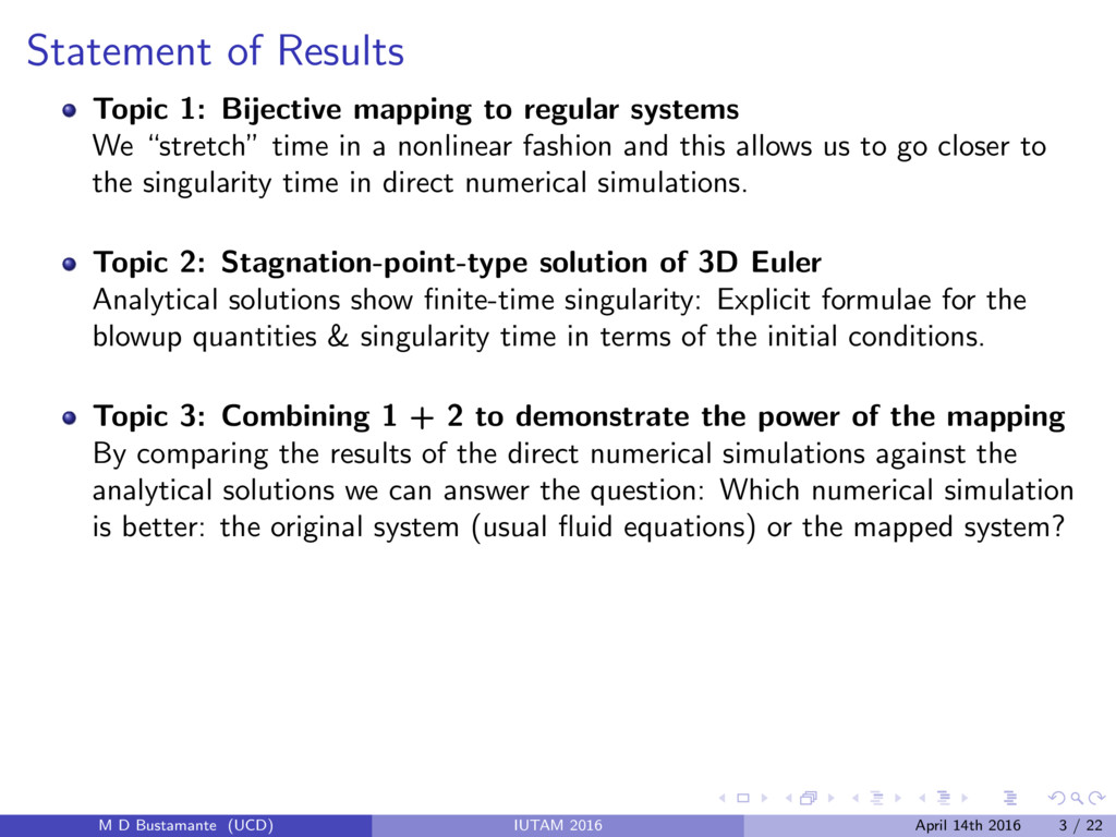
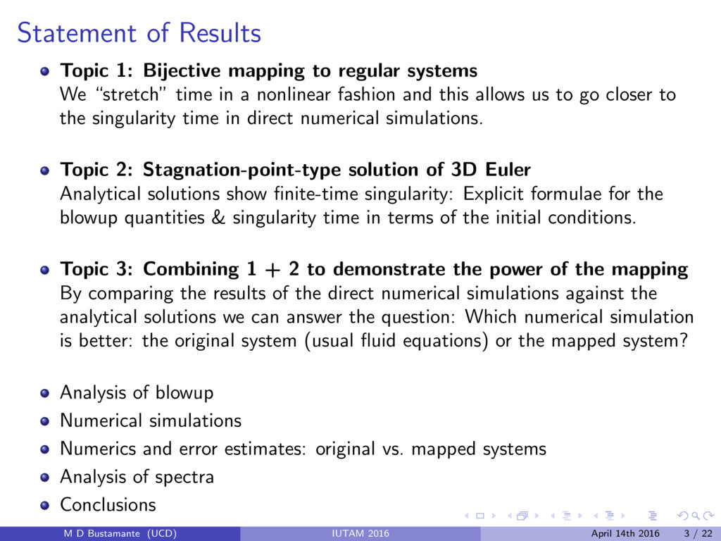
4. Statement of Results Topic 1: Bijective mapping to regular systems We “stretch” time in a nonlinear fashion and this allows us to go closer to the singularity time in direct numerical simulations. Topic 2: Stagnation-point-type solution of 3D Euler Analytical solutions show finite-time singularity: Explicit formulae for the blowup quantities & singularity time in terms of the initial conditions. Topic 3: Combining 1 + 2 to demonstrate the power of the mapping By comparing the results of the direct numerical simulations against the analytical solutions we can answer the question: Which numerical simulation is better: the original system (usual fluid equations) or the mapped system? M D Bustamante (UCD) IUTAM 2016 April 14th 2016 3 / 22
5. Statement of Results Topic 1: Bijective mapping to regular systems We “stretch” time in a nonlinear fashion and this allows us to go closer to the singularity time in direct numerical simulations. Topic 2: Stagnation-point-type solution of 3D Euler Analytical solutions show finite-time singularity: Explicit formulae for the blowup quantities & singularity time in terms of the initial conditions. Topic 3: Combining 1 + 2 to demonstrate the power of the mapping By comparing the results of the direct numerical simulations against the analytical solutions we can answer the question: Which numerical simulation is better: the original system (usual fluid equations) or the mapped system? Analysis of blowup Numerical simulations Numerics and error estimates: original vs. mapped systems Analysis of spectra Conclusions M D Bustamante (UCD) IUTAM 2016 April 14th 2016 3 / 22
6. Topic 1: Mapping to regular systems M D Bustamante (UCD) IUTAM 2016 April 14th 2016 4 / 22
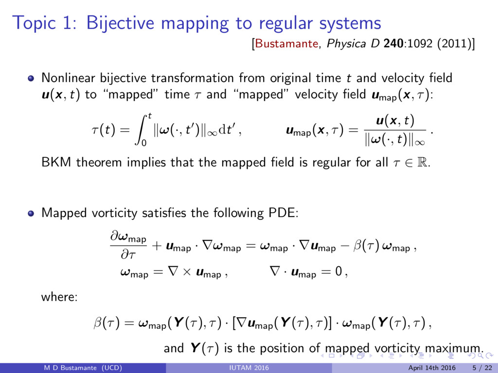
7. Topic 1: Bijective mapping to regular systems [Bustamante, Physica D 240:1092 (2011)] Nonlinear bijective transformation from original time t and velocity field u ( x , t) to “mapped” time ⌧ and “mapped” velocity field umap ( x , ⌧): ⌧(t) = Z t 0 k!(·, t0)k1dt0 , umap ( x , ⌧) = u ( x , t) k!(·, t)k1 . BKM theorem implies that the mapped field is regular for all ⌧ 2 R. M D Bustamante (UCD) IUTAM 2016 April 14th 2016 5 / 22
8. Topic 1: Bijective mapping to regular systems [Bustamante, Physica D 240:1092 (2011)] Nonlinear bijective transformation from original time t and velocity field u ( x , t) to “mapped” time ⌧ and “mapped” velocity field umap ( x , ⌧): ⌧(t) = Z t 0 k!(·, t0)k1dt0 , umap ( x , ⌧) = u ( x , t) k!(·, t)k1 . BKM theorem implies that the mapped field is regular for all ⌧ 2 R. Mapped vorticity satisfies the following PDE: @! map @⌧ + umap · r! map = ! map · r umap (⌧) ! map , ! map = r ⇥ umap , r · umap = 0 , where: (⌧) = ! map ( Y (⌧), ⌧) · [r umap ( Y (⌧), ⌧)] · ! map ( Y (⌧), ⌧) , and Y (⌧) is the position of mapped vorticity maximum. M D Bustamante (UCD) IUTAM 2016 April 14th 2016 5 / 22
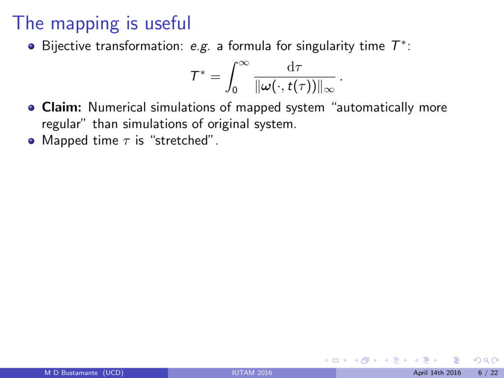
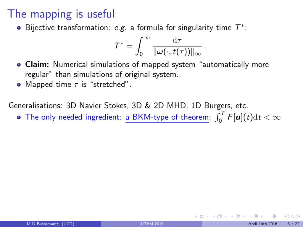
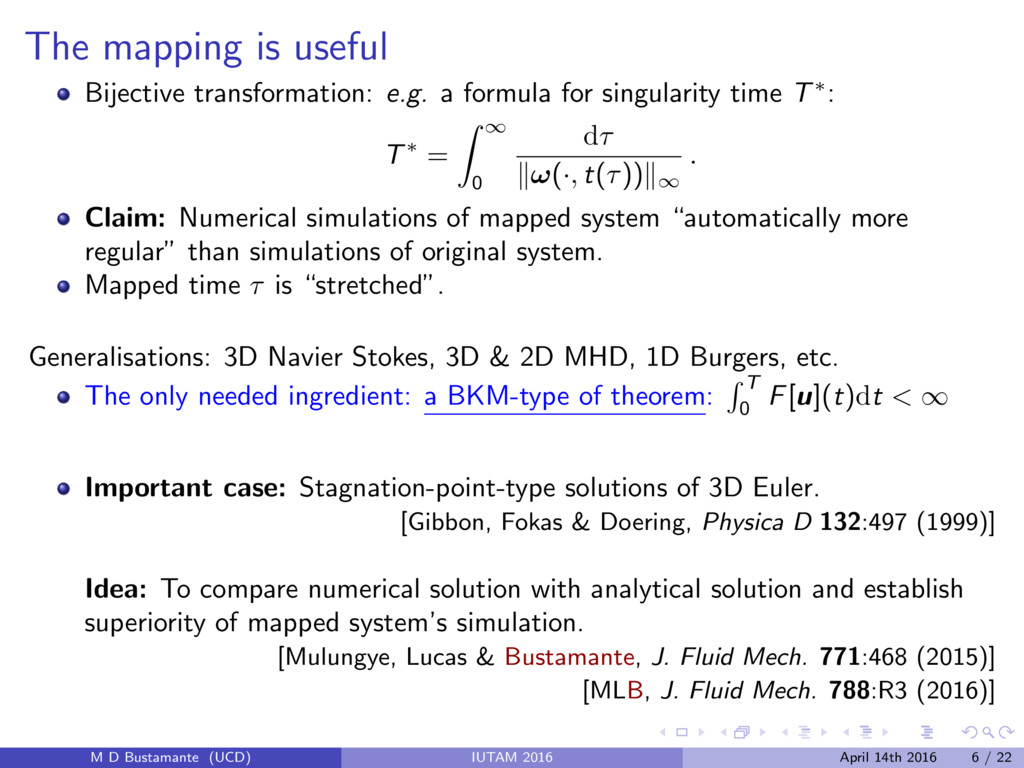
9. The mapping is useful Bijective transformation: e.g. a formula for singularity time T⇤: T⇤ = Z 1 0 d⌧ k!(·, t(⌧))k1 . Claim: Numerical simulations of mapped system “automatically more regular” than simulations of original system. Mapped time ⌧ is “stretched”. M D Bustamante (UCD) IUTAM 2016 April 14th 2016 6 / 22
10. The mapping is useful Bijective transformation: e.g. a formula for singularity time T⇤: T⇤ = Z 1 0 d⌧ k!(·, t(⌧))k1 . Claim: Numerical simulations of mapped system “automatically more regular” than simulations of original system. Mapped time ⌧ is “stretched”. Generalisations: 3D Navier Stokes, 3D & 2D MHD, 1D Burgers, etc. The only needed ingredient: a BKM-type of theorem: R T 0 F[ u ](t)dt < 1 M D Bustamante (UCD) IUTAM 2016 April 14th 2016 6 / 22
11. The mapping is useful Bijective transformation: e.g. a formula for singularity time T⇤: T⇤ = Z 1 0 d⌧ k!(·, t(⌧))k1 . Claim: Numerical simulations of mapped system “automatically more regular” than simulations of original system. Mapped time ⌧ is “stretched”. Generalisations: 3D Navier Stokes, 3D & 2D MHD, 1D Burgers, etc. The only needed ingredient: a BKM-type of theorem: R T 0 F[ u ](t)dt < 1 Important case: Stagnation-point-type solutions of 3D Euler. [Gibbon, Fokas & Doering, Physica D 132:497 (1999)] Idea: To compare numerical solution with analytical solution and establish superiority of mapped system’s simulation. [Mulungye, Lucas & Bustamante, J. Fluid Mech. 771:468 (2015)] [MLB, J. Fluid Mech. 788:R3 (2016)] M D Bustamante (UCD) IUTAM 2016 April 14th 2016 6 / 22
12. Topic 2: Stagnation-point-type solutions of 3D Euler M D Bustamante (UCD) IUTAM 2016 April 14th 2016 7 / 22
13. 3D Euler on a discrete symmetry plane Most 3D Euler numerical simulations exploit discrete reflection symmetries: Taylor-Green: 6 symmetry planes. Kida-Pelz: 6 symmetry planes. Kerr’s anti-parallel vortices: 4 symmetry planes. Simplest case: 1 symmetry plane (along non-periodic direction). M D Bustamante (UCD) IUTAM 2016 April 14th 2016 8 / 22
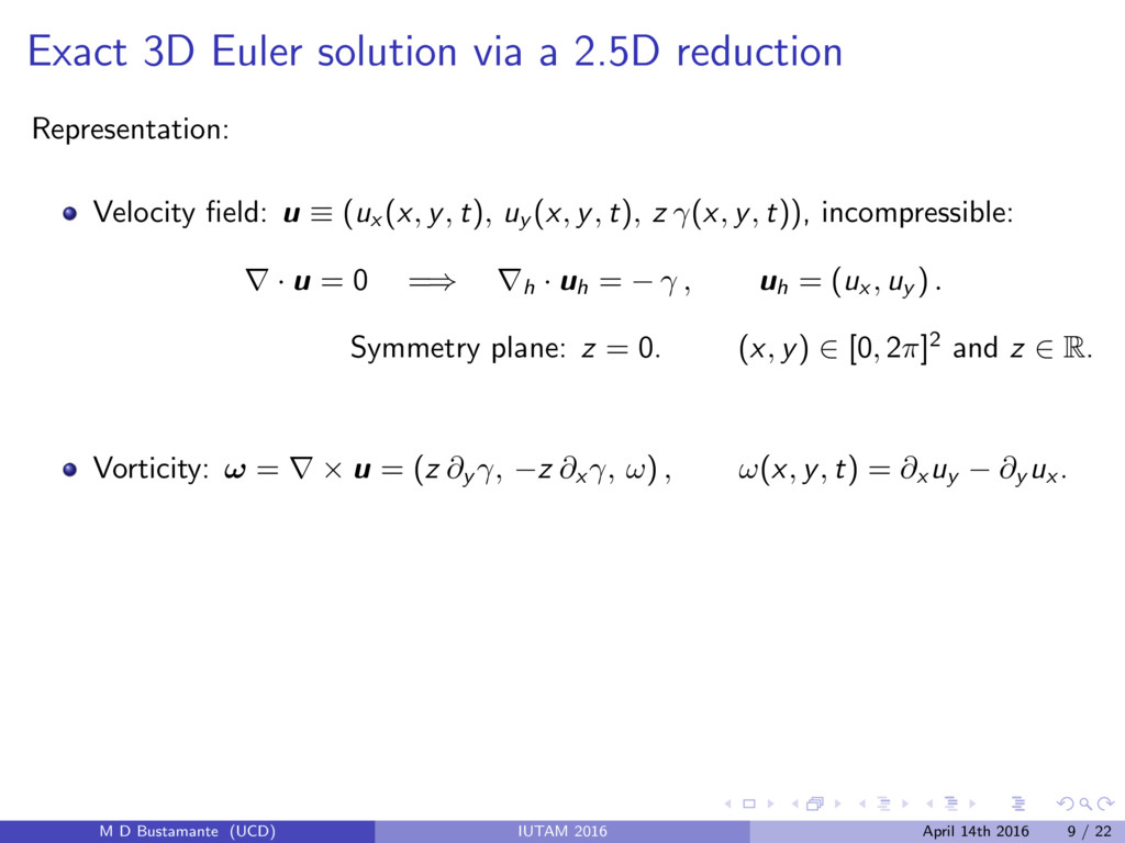
14. Exact 3D Euler solution via a 2.5D reduction Representation: Velocity field: u ⌘ (u x (x, y, t), u y (x, y, t), z (x, y, t)), incompressible: r · u = 0 =) r h · uh = , uh = (u x , u y ) . Symmetry plane: z = 0. (x, y) 2 [0, 2⇡]2 and z 2 R. M D Bustamante (UCD) IUTAM 2016 April 14th 2016 9 / 22
15. Exact 3D Euler solution via a 2.5D reduction Representation: Velocity field: u ⌘ (u x (x, y, t), u y (x, y, t), z (x, y, t)), incompressible: r · u = 0 =) r h · uh = , uh = (u x , u y ) . Symmetry plane: z = 0. (x, y) 2 [0, 2⇡]2 and z 2 R. Vorticity: ! = r ⇥ u = (z @ y , z @ x , !) , !(x, y, t) = @ x u y @ y u x . M D Bustamante (UCD) IUTAM 2016 April 14th 2016 9 / 22
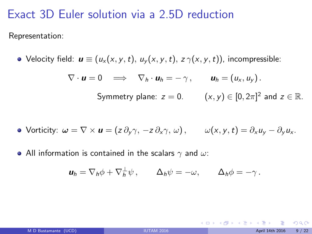
16. Exact 3D Euler solution via a 2.5D reduction Representation: Velocity field: u ⌘ (u x (x, y, t), u y (x, y, t), z (x, y, t)), incompressible: r · u = 0 =) r h · uh = , uh = (u x , u y ) . Symmetry plane: z = 0. (x, y) 2 [0, 2⇡]2 and z 2 R. Vorticity: ! = r ⇥ u = (z @ y , z @ x , !) , !(x, y, t) = @ x u y @ y u x . All information is contained in the scalars and !: uh = r h + r? h , h = !, h = . M D Bustamante (UCD) IUTAM 2016 April 14th 2016 9 / 22
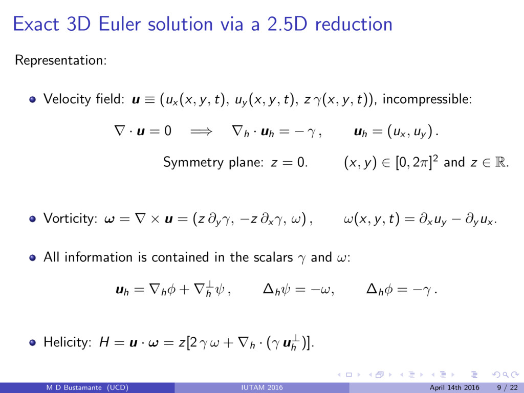
17. Exact 3D Euler solution via a 2.5D reduction Representation: Velocity field: u ⌘ (u x (x, y, t), u y (x, y, t), z (x, y, t)), incompressible: r · u = 0 =) r h · uh = , uh = (u x , u y ) . Symmetry plane: z = 0. (x, y) 2 [0, 2⇡]2 and z 2 R. Vorticity: ! = r ⇥ u = (z @ y , z @ x , !) , !(x, y, t) = @ x u y @ y u x . All information is contained in the scalars and !: uh = r h + r? h , h = !, h = . Helicity: H = u · ! = z[2 ! + r h · ( u ? h )]. M D Bustamante (UCD) IUTAM 2016 April 14th 2016 9 / 22
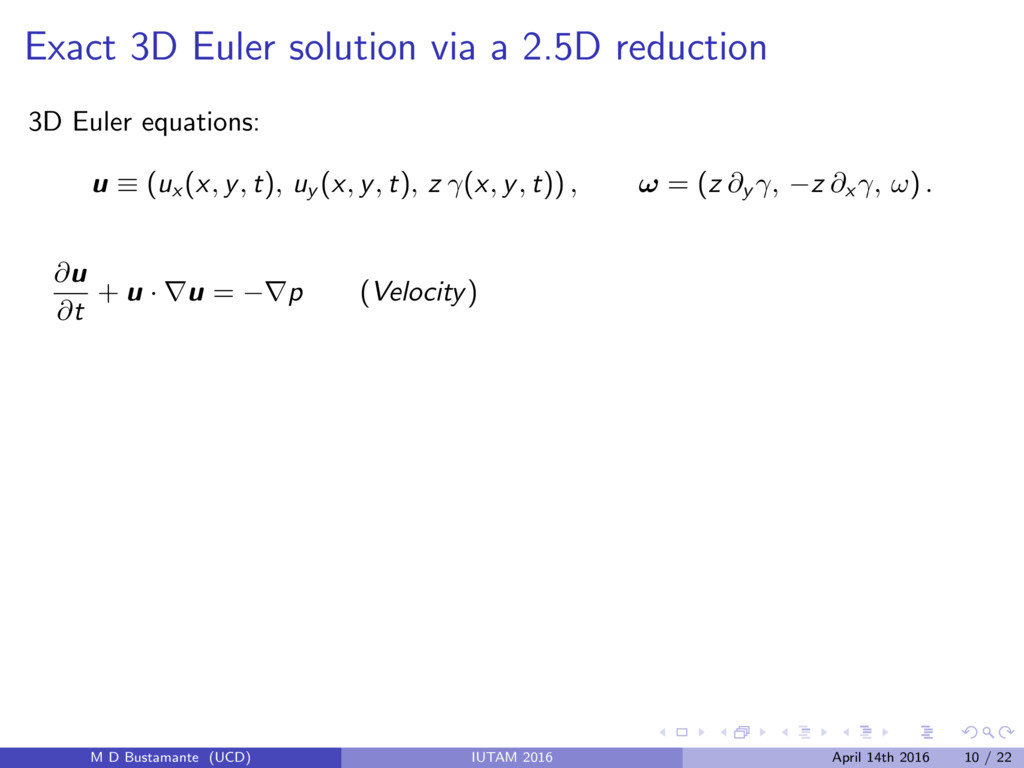
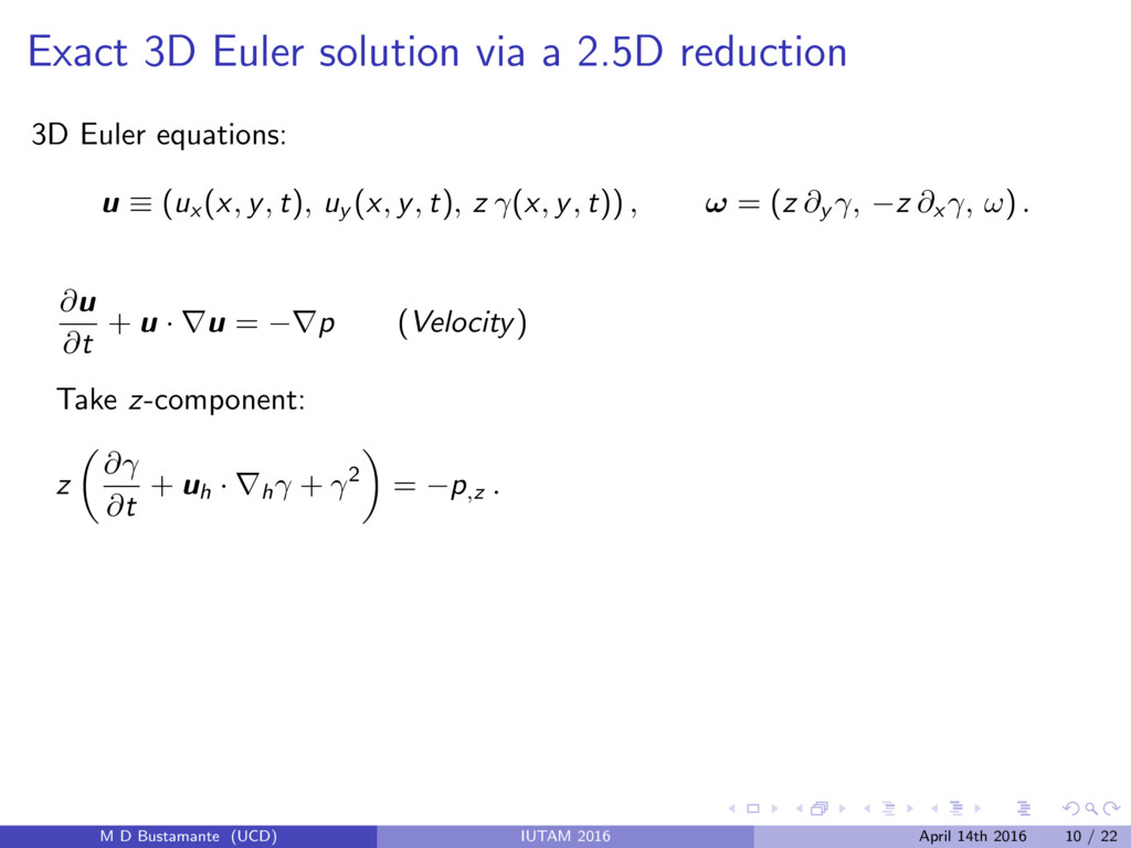
18. Exact 3D Euler solution via a 2.5D reduction 3D Euler equations: u ⌘ (u x (x, y, t), u y (x, y, t), z (x, y, t)) , ! = (z @ y , z @ x , !) . @ u @t + u · r u = rp (Velocity) M D Bustamante (UCD) IUTAM 2016 April 14th 2016 10 / 22
19. Exact 3D Euler solution via a 2.5D reduction 3D Euler equations: u ⌘ (u x (x, y, t), u y (x, y, t), z (x, y, t)) , ! = (z @ y , z @ x , !) . @ u @t + u · r u = rp (Velocity) Take z-component: z ✓ @ @t + uh · r h + 2 ◆ = p, z . M D Bustamante (UCD) IUTAM 2016 April 14th 2016 10 / 22
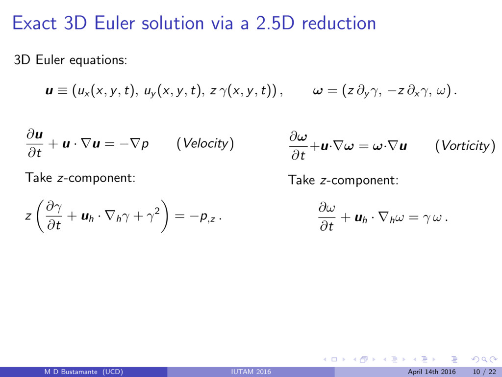
20. Exact 3D Euler solution via a 2.5D reduction 3D Euler equations: u ⌘ (u x (x, y, t), u y (x, y, t), z (x, y, t)) , ! = (z @ y , z @ x , !) . @ u @t + u · r u = rp (Velocity) Take z-component: z ✓ @ @t + uh · r h + 2 ◆ = p, z . @! @t + u ·r! = !·r u (Vorticity) M D Bustamante (UCD) IUTAM 2016 April 14th 2016 10 / 22
21. Exact 3D Euler solution via a 2.5D reduction 3D Euler equations: u ⌘ (u x (x, y, t), u y (x, y, t), z (x, y, t)) , ! = (z @ y , z @ x , !) . @ u @t + u · r u = rp (Velocity) Take z-component: z ✓ @ @t + uh · r h + 2 ◆ = p, z . @! @t + u ·r! = !·r u (Vorticity) Take z-component: @! @t + uh · r h ! = ! . M D Bustamante (UCD) IUTAM 2016 April 14th 2016 10 / 22
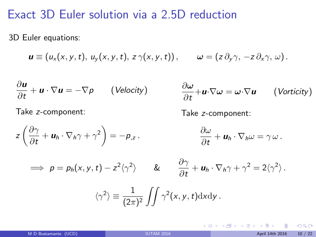
22. Exact 3D Euler solution via a 2.5D reduction 3D Euler equations: u ⌘ (u x (x, y, t), u y (x, y, t), z (x, y, t)) , ! = (z @ y , z @ x , !) . @ u @t + u · r u = rp (Velocity) Take z-component: z ✓ @ @t + uh · r h + 2 ◆ = p, z . @! @t + u ·r! = !·r u (Vorticity) Take z-component: @! @t + uh · r h ! = ! . =) p = p h (x, y, t) z2h 2i & @ @t + uh · r h + 2 = 2h 2i . h 2i ⌘ 1 (2⇡)2 ZZ 2(x, y, t)dxdy . M D Bustamante (UCD) IUTAM 2016 April 14th 2016 10 / 22
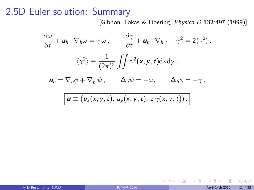
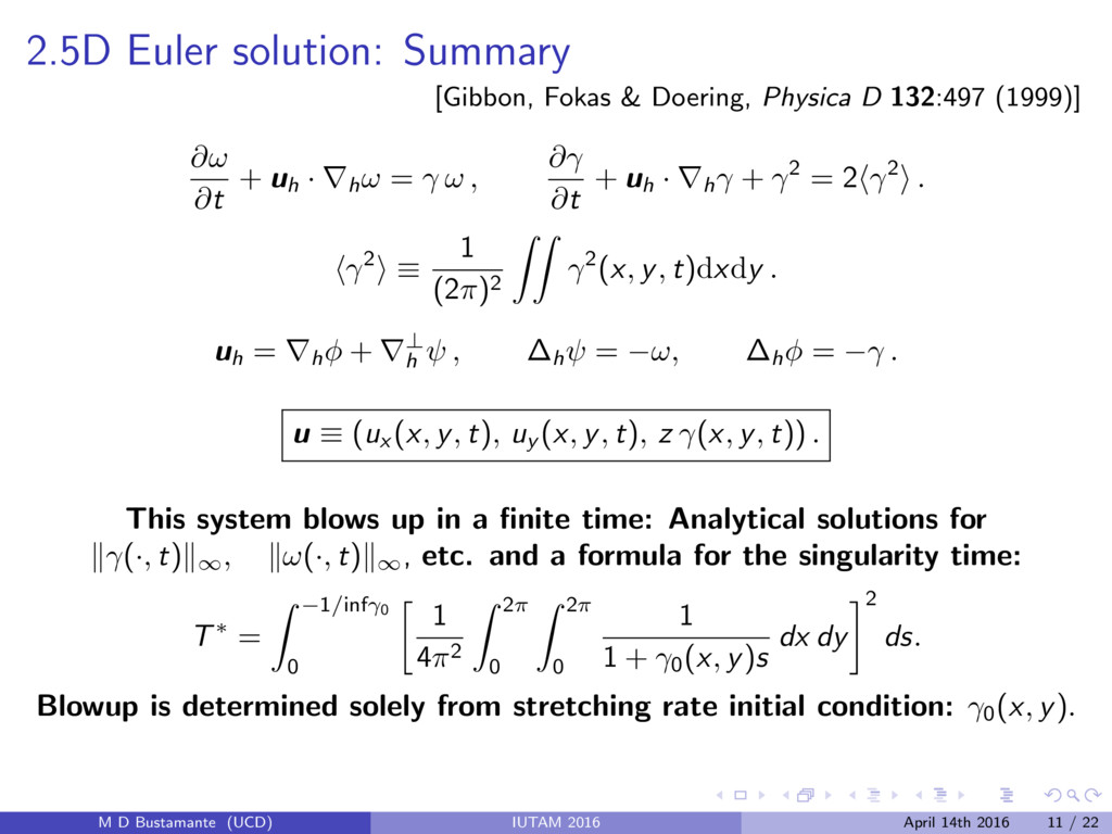
23. 2.5D Euler solution: Summary [Gibbon, Fokas & Doering, Physica D 132:497 (1999)] @! @t + uh · r h ! = ! , @ @t + uh · r h + 2 = 2h 2i . h 2i ⌘ 1 (2⇡)2 ZZ 2(x, y, t)dxdy . uh = r h + r? h , h = !, h = . u ⌘ (u x (x, y, t), u y (x, y, t), z (x, y, t)) . M D Bustamante (UCD) IUTAM 2016 April 14th 2016 11 / 22
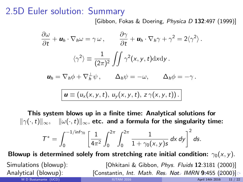
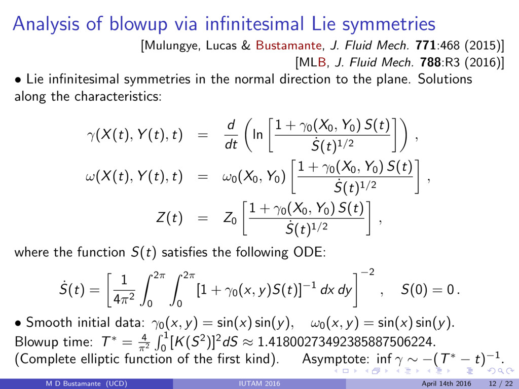
24. 2.5D Euler solution: Summary [Gibbon, Fokas & Doering, Physica D 132:497 (1999)] @! @t + uh · r h ! = ! , @ @t + uh · r h + 2 = 2h 2i . h 2i ⌘ 1 (2⇡)2 ZZ 2(x, y, t)dxdy . uh = r h + r? h , h = !, h = . u ⌘ (u x (x, y, t), u y (x, y, t), z (x, y, t)) . This system blows up in a finite time: Analytical solutions for k (·, t)k1, k!(·, t)k1 , etc. and a formula for the singularity time: T⇤ = Z 1 / inf 0 0  1 4⇡2 Z 2 ⇡ 0 Z 2 ⇡ 0 1 1 + 0 (x, y)s dx dy 2 ds. Blowup is determined solely from stretching rate initial condition: 0 (x, y). M D Bustamante (UCD) IUTAM 2016 April 14th 2016 11 / 22
25. 2.5D Euler solution: Summary [Gibbon, Fokas & Doering, Physica D 132:497 (1999)] @! @t + uh · r h ! = ! , @ @t + uh · r h + 2 = 2h 2i . h 2i ⌘ 1 (2⇡)2 ZZ 2(x, y, t)dxdy . uh = r h + r? h , h = !, h = . u ⌘ (u x (x, y, t), u y (x, y, t), z (x, y, t)) . This system blows up in a finite time: Analytical solutions for k (·, t)k1, k!(·, t)k1 , etc. and a formula for the singularity time: T⇤ = Z 1 / inf 0 0  1 4⇡2 Z 2 ⇡ 0 Z 2 ⇡ 0 1 1 + 0 (x, y)s dx dy 2 ds. Blowup is determined solely from stretching rate initial condition: 0 (x, y). Simulations (blowup): [Ohkitani & Gibbon, Phys. Fluids 12:3181 (2000)] Analytical (blowup): [Constantin, Int. Math. Res. Not. IMRN 9:455 (2000)] M D Bustamante (UCD) IUTAM 2016 April 14th 2016 11 / 22
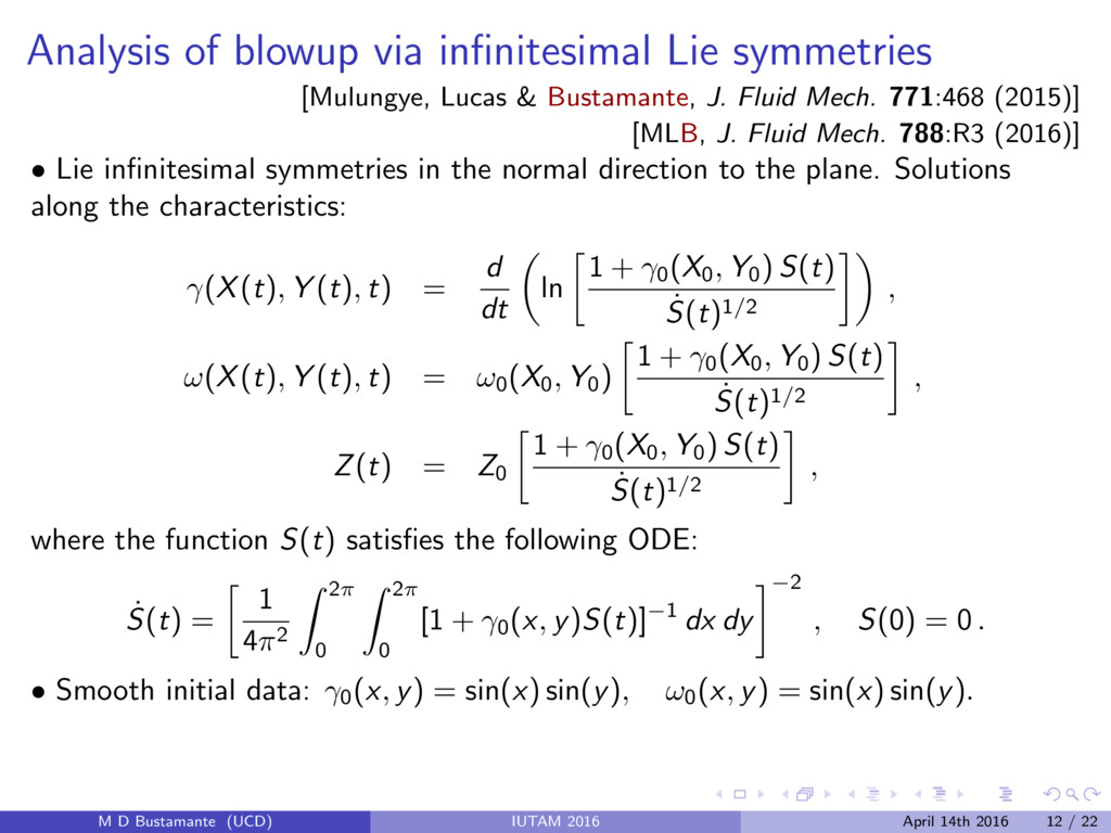
26. Analysis of blowup via infinitesimal Lie symmetries [Mulungye, Lucas & Bustamante, J. Fluid Mech. 771:468 (2015)] [MLB, J. Fluid Mech. 788:R3 (2016)] • Lie infinitesimal symmetries in the normal direction to the plane. Solutions along the characteristics: M D Bustamante (UCD) IUTAM 2016 April 14th 2016 12 / 22
27. Analysis of blowup via infinitesimal Lie symmetries [Mulungye, Lucas & Bustamante, J. Fluid Mech. 771:468 (2015)] [MLB, J. Fluid Mech. 788:R3 (2016)] • Lie infinitesimal symmetries in the normal direction to the plane. Solutions along the characteristics: (X(t), Y (t), t) = d dt ✓ ln  1 + 0 (X 0 , Y 0 ) S(t) ˙ S(t)1 / 2 ◆ , !(X(t), Y (t), t) = ! 0 (X 0 , Y 0 )  1 + 0 (X 0 , Y 0 ) S(t) ˙ S(t)1 / 2 , Z(t) = Z 0  1 + 0 (X 0 , Y 0 ) S(t) ˙ S(t)1 / 2 , where the function S(t) satisfies the following ODE: ˙ S(t) =  1 4⇡2 Z 2 ⇡ 0 Z 2 ⇡ 0 [1 + 0 (x, y)S(t)] 1 dx dy 2 , S(0) = 0 . • Smooth initial data: 0 (x, y) = sin(x) sin(y), ! 0 (x, y) = sin(x) sin(y). M D Bustamante (UCD) IUTAM 2016 April 14th 2016 12 / 22
28. Analysis of blowup via infinitesimal Lie symmetries [Mulungye, Lucas & Bustamante, J. Fluid Mech. 771:468 (2015)] [MLB, J. Fluid Mech. 788:R3 (2016)] • Lie infinitesimal symmetries in the normal direction to the plane. Solutions along the characteristics: (X(t), Y (t), t) = d dt ✓ ln  1 + 0 (X 0 , Y 0 ) S(t) ˙ S(t)1 / 2 ◆ , !(X(t), Y (t), t) = ! 0 (X 0 , Y 0 )  1 + 0 (X 0 , Y 0 ) S(t) ˙ S(t)1 / 2 , Z(t) = Z 0  1 + 0 (X 0 , Y 0 ) S(t) ˙ S(t)1 / 2 , where the function S(t) satisfies the following ODE: ˙ S(t) =  1 4⇡2 Z 2 ⇡ 0 Z 2 ⇡ 0 [1 + 0 (x, y)S(t)] 1 dx dy 2 , S(0) = 0 . • Smooth initial data: 0 (x, y) = sin(x) sin(y), ! 0 (x, y) = sin(x) sin(y). Blowup time: T⇤ = 4 ⇡2 R 1 0 [K(S2 )]2 dS ⇡ 1.41800273492385887506224. (Complete elliptic function of the first kind). Asymptote: inf ⇠ (T⇤ t) 1. M D Bustamante (UCD) IUTAM 2016 April 14th 2016 12 / 22
29. There is a Beale-Kato-Majda type of theorem [Gibbon & Ohkitani, Nonlinearity 14:1239 (2001)] R t 0 k (·, t0)k1dt0 < 1 criterion for regularity. M D Bustamante (UCD) IUTAM 2016 April 14th 2016 13 / 22
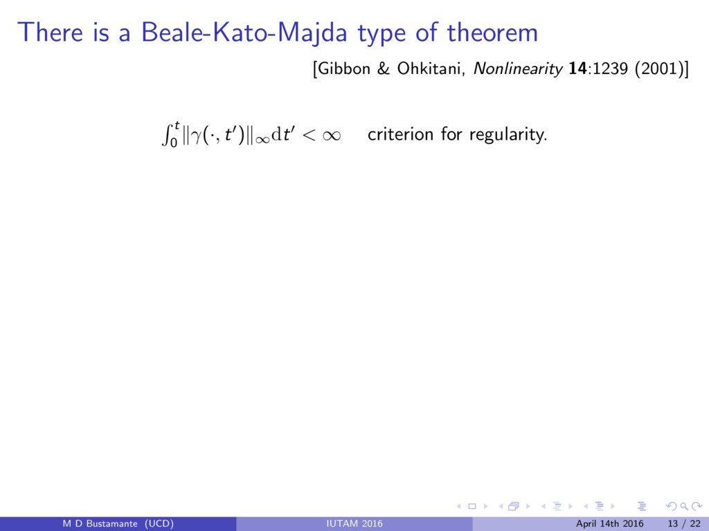
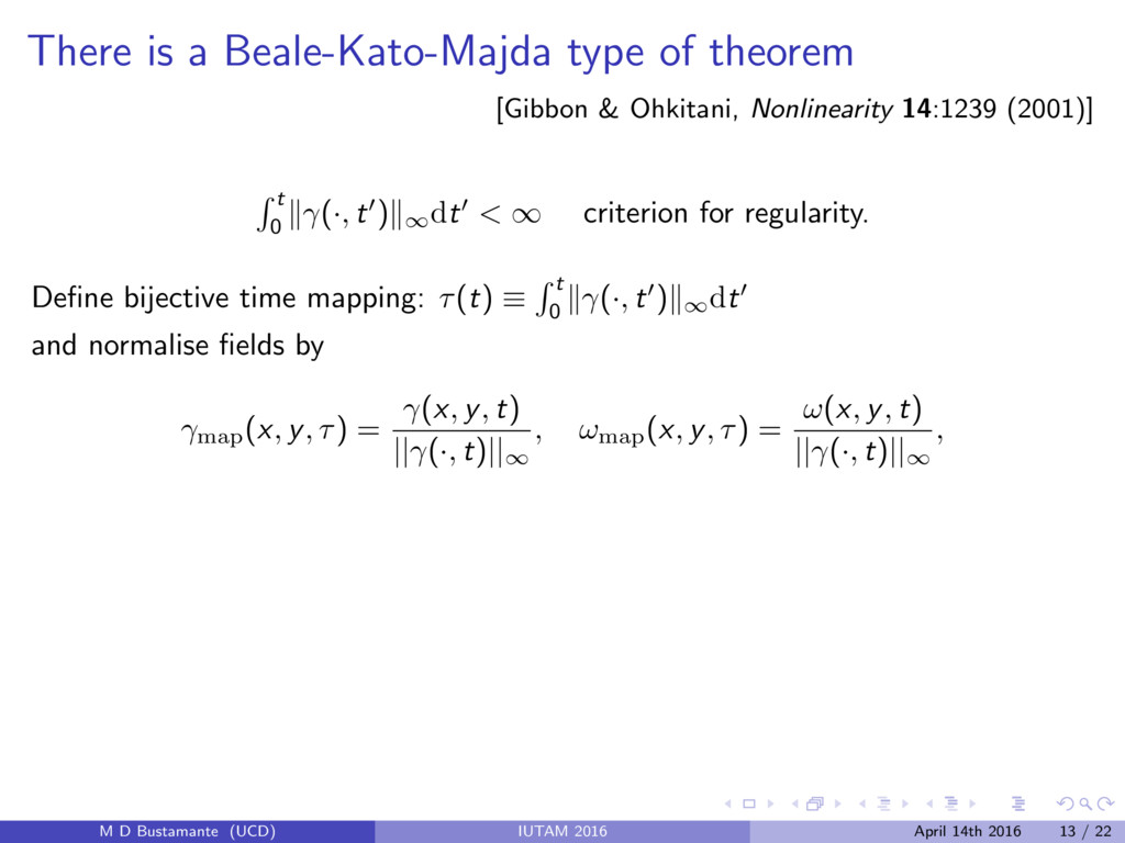
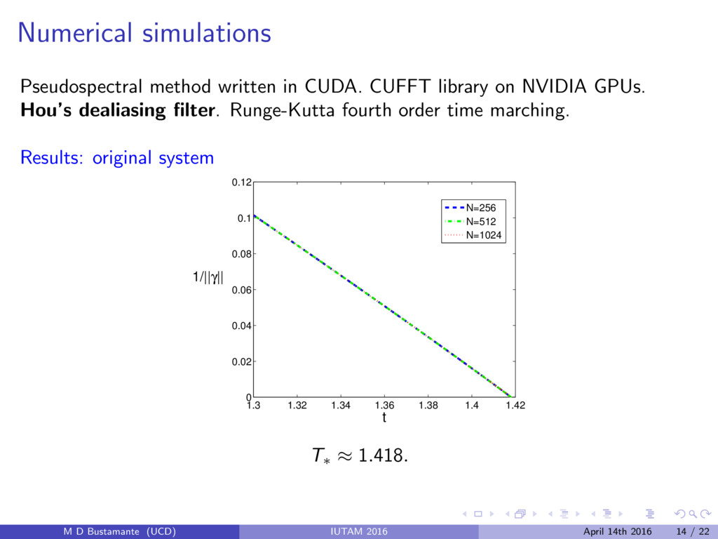
30. There is a Beale-Kato-Majda type of theorem [Gibbon & Ohkitani, Nonlinearity 14:1239 (2001)] R t 0 k (·, t0)k1dt0 < 1 criterion for regularity. Define bijective time mapping: ⌧(t) ⌘ R t 0 k (·, t0)k1dt0 and normalise fields by map (x, y, ⌧) = (x, y, t) || (·, t)||1 , !map (x, y, ⌧) = !(x, y, t) || (·, t)||1 , M D Bustamante (UCD) IUTAM 2016 April 14th 2016 13 / 22
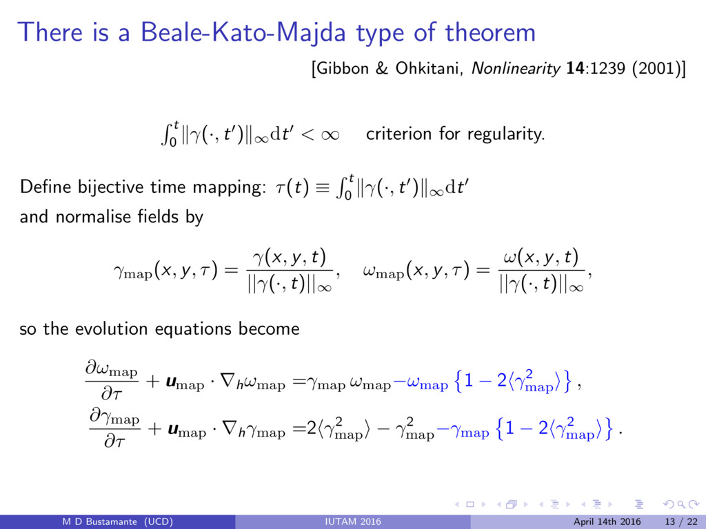
31. There is a Beale-Kato-Majda type of theorem [Gibbon & Ohkitani, Nonlinearity 14:1239 (2001)] R t 0 k (·, t0)k1dt0 < 1 criterion for regularity. Define bijective time mapping: ⌧(t) ⌘ R t 0 k (·, t0)k1dt0 and normalise fields by map (x, y, ⌧) = (x, y, t) || (·, t)||1 , !map (x, y, ⌧) = !(x, y, t) || (·, t)||1 , so the evolution equations become @!map @⌧ + umap · r h !map = map !map !map 1 2h 2 map i , @ map @⌧ + umap · r h map =2h 2 map i 2 map map 1 2h 2 map i . M D Bustamante (UCD) IUTAM 2016 April 14th 2016 13 / 22
32. Numerical simulations Pseudospectral method written in CUDA. CUFFT library on NVIDIA GPUs. Hou’s dealiasing filter. Runge-Kutta fourth order time marching. Results: original system 1.3 1.32 1.34 1.36 1.38 1.4 1.42 0 0.02 0.04 0.06 0.08 0.1 0.12 1/||γ|| t N=256 N=512 N=1024 T⇤ ⇡ 1.418. M D Bustamante (UCD) IUTAM 2016 April 14th 2016 14 / 22
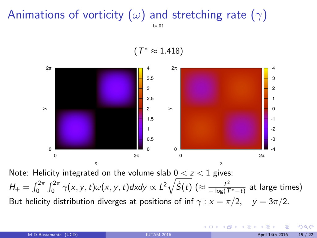
33. Animations of vorticity (!) and stretching rate ( ) (T⇤ ⇡ 1.418) Note: Helicity integrated on the volume slab 0 < z < 1 gives: H + = R 2 ⇡ 0 R 2 ⇡ 0 (x, y, t)!(x, y, t)dxdy / L2 q ˙ S(t) (⇡ L2 log(T ⇤ t) at large times) But helicity distribution diverges at positions of inf : x = ⇡/2, y = 3⇡/2. M D Bustamante (UCD) IUTAM 2016 April 14th 2016 15 / 22
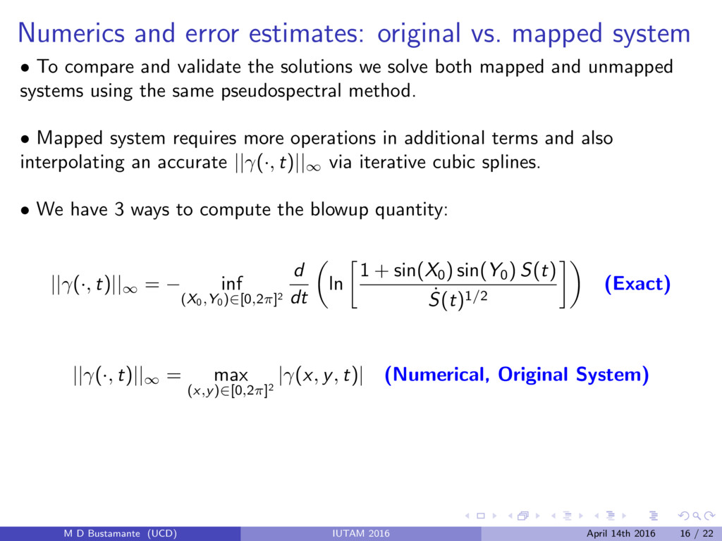
34. Numerics and error estimates: original vs. mapped system • To compare and validate the solutions we solve both mapped and unmapped systems using the same pseudospectral method. M D Bustamante (UCD) IUTAM 2016 April 14th 2016 16 / 22
35. Numerics and error estimates: original vs. mapped system • To compare and validate the solutions we solve both mapped and unmapped systems using the same pseudospectral method. • Mapped system requires more operations in additional terms and also interpolating an accurate || (·, t)||1 via iterative cubic splines. M D Bustamante (UCD) IUTAM 2016 April 14th 2016 16 / 22
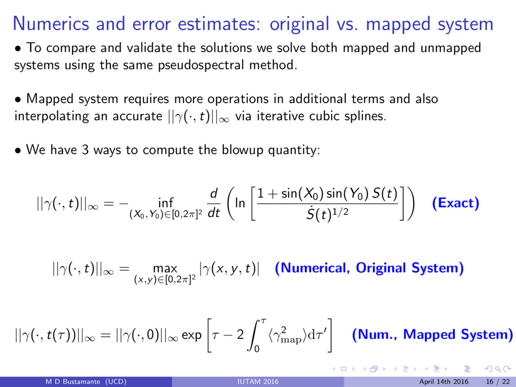
36. Numerics and error estimates: original vs. mapped system • To compare and validate the solutions we solve both mapped and unmapped systems using the same pseudospectral method. • Mapped system requires more operations in additional terms and also interpolating an accurate || (·, t)||1 via iterative cubic splines. • We have 3 ways to compute the blowup quantity: || (·, t)||1 = inf (X0 , Y0) 2 [0 , 2 ⇡ ]2 d dt ✓ ln  1 + sin(X 0 ) sin(Y 0 ) S(t) ˙ S(t)1 / 2 ◆ (Exact) M D Bustamante (UCD) IUTAM 2016 April 14th 2016 16 / 22
37. Numerics and error estimates: original vs. mapped system • To compare and validate the solutions we solve both mapped and unmapped systems using the same pseudospectral method. • Mapped system requires more operations in additional terms and also interpolating an accurate || (·, t)||1 via iterative cubic splines. • We have 3 ways to compute the blowup quantity: || (·, t)||1 = inf (X0 , Y0) 2 [0 , 2 ⇡ ]2 d dt ✓ ln  1 + sin(X 0 ) sin(Y 0 ) S(t) ˙ S(t)1 / 2 ◆ (Exact) || (·, t)||1 = max (x , y) 2 [0 , 2 ⇡ ]2 | (x, y, t)| (Numerical, Original System) M D Bustamante (UCD) IUTAM 2016 April 14th 2016 16 / 22
38. Numerics and error estimates: original vs. mapped system • To compare and validate the solutions we solve both mapped and unmapped systems using the same pseudospectral method. • Mapped system requires more operations in additional terms and also interpolating an accurate || (·, t)||1 via iterative cubic splines. • We have 3 ways to compute the blowup quantity: || (·, t)||1 = inf (X0 , Y0) 2 [0 , 2 ⇡ ]2 d dt ✓ ln  1 + sin(X 0 ) sin(Y 0 ) S(t) ˙ S(t)1 / 2 ◆ (Exact) || (·, t)||1 = max (x , y) 2 [0 , 2 ⇡ ]2 | (x, y, t)| (Numerical, Original System) || (·, t(⌧))||1 = || (·, 0)||1 exp  ⌧ 2 Z ⌧ 0 h 2 map id⌧0 (Num., Mapped System) M D Bustamante (UCD) IUTAM 2016 April 14th 2016 16 / 22
39. Errors wrt analytical solution reveal a machine-epsilon barrier for original system simulation (T⇤ t ⇡ 10 16) Q(f , g) = kf gk 2 kf k 2 + kgk 2 (0  Q  1). L2 -norm is computed over simulation time. 10 18 10 16 10 14 10 12 10 10 10 08 10 06 0.0001 0.01 1 0 5 10 15 20 25 30 35 40 Q ⌧ d⌧ = 2.5 ⇥ 10 3 d⌧ = 10 3 d⌧ = 10 4 d⌧ = 10 3 mapped d⌧ = 10 4 mapped d⌧ = 10 5 mapped Figure: Time evolution of the error measures Q = Q (k num (·, t )k1, k ana (·, t )k1 ), showing the convergence with time step d ⌧. M D Bustamante (UCD) IUTAM 2016 April 14th 2016 17 / 22
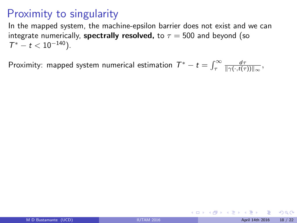
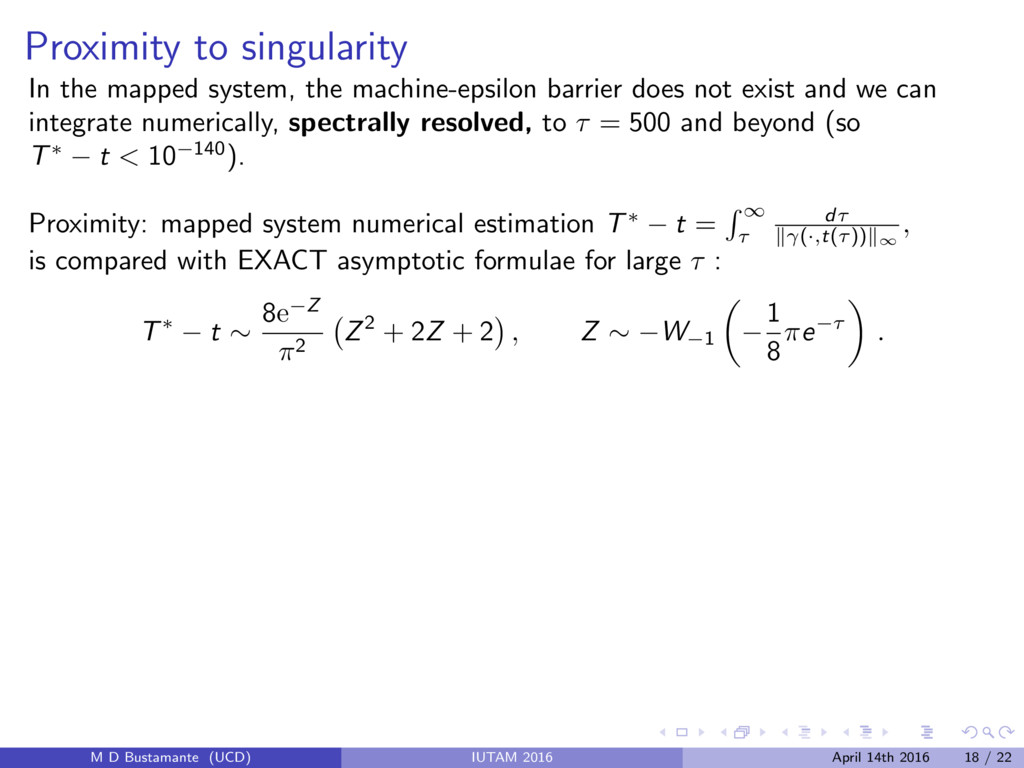
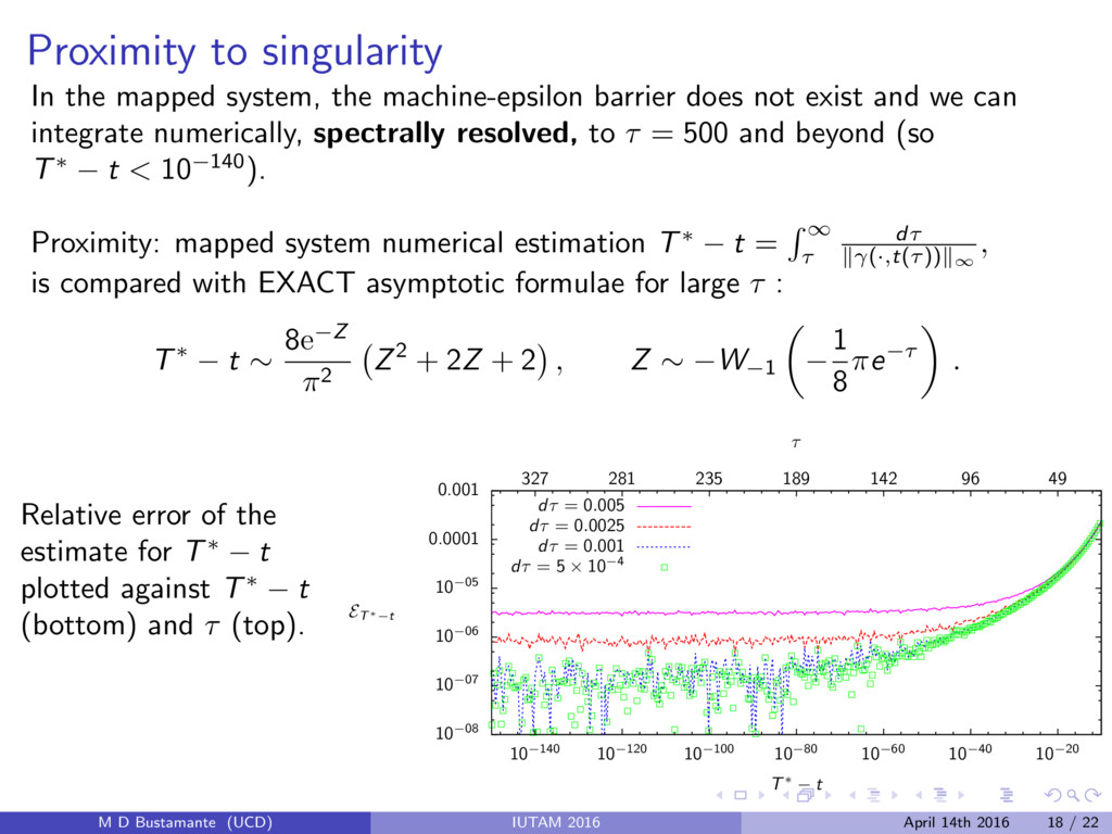
40. Proximity to singularity In the mapped system, the machine-epsilon barrier does not exist and we can integrate numerically, spectrally resolved, to ⌧ = 500 and beyond (so T⇤ t < 10 140 ). Proximity: mapped system numerical estimation T⇤ t = R 1 ⌧ d ⌧ k ( ·, t( ⌧ )) k1 , M D Bustamante (UCD) IUTAM 2016 April 14th 2016 18 / 22
41. Proximity to singularity In the mapped system, the machine-epsilon barrier does not exist and we can integrate numerically, spectrally resolved, to ⌧ = 500 and beyond (so T⇤ t < 10 140 ). Proximity: mapped system numerical estimation T⇤ t = R 1 ⌧ d ⌧ k ( ·, t( ⌧ )) k1 , is compared with EXACT asymptotic formulae for large ⌧ : T⇤ t ⇠ 8e Z ⇡2 Z2 + 2Z + 2 , Z ⇠ W 1 ✓ 1 8 ⇡e ⌧ ◆ . M D Bustamante (UCD) IUTAM 2016 April 14th 2016 18 / 22
42. Proximity to singularity In the mapped system, the machine-epsilon barrier does not exist and we can integrate numerically, spectrally resolved, to ⌧ = 500 and beyond (so T⇤ t < 10 140 ). Proximity: mapped system numerical estimation T⇤ t = R 1 ⌧ d ⌧ k ( ·, t( ⌧ )) k1 , is compared with EXACT asymptotic formulae for large ⌧ : T⇤ t ⇠ 8e Z ⇡2 Z2 + 2Z + 2 , Z ⇠ W 1 ✓ 1 8 ⇡e ⌧ ◆ . Relative error of the estimate for T⇤ t plotted against T⇤ t (bottom) and ⌧ (top). 10 08 10 07 10 06 10 05 0.0001 0.001 10 140 327 10 120 281 10 100 235 10 80 189 10 60 142 10 40 96 10 20 49 E T ⇤ t T⇤ t ⌧ d⌧ = 0.005 d⌧ = 0.0025 d⌧ = 0.001 d⌧ = 5 ⇥ 10 4 M D Bustamante (UCD) IUTAM 2016 April 14th 2016 18 / 22
43. Early spectra: Transient burst of energy Early spectra: ‘usual’ exponential decay E(k, t) ⇡ C(t)k n(t) exp( 2 (t)k). 10 40 10 35 10 30 10 25 10 20 10 15 10 10 10 05 1 0 200 400 600 800 100012001400160018002000 E(k) ⌧ = 5 t = 1.396 T⇤ t ⇡ 0.022 N = 4096 ⌫ = 2 ⇥ 10 10 N = 4096 ⌫ = 0 N = 1024 ⌫ = 0 N = 1024 ⌫ = 10 10 10 40 10 35 10 30 10 25 10 20 10 15 10 10 10 05 1 50 100 150 200 250 300 350 400 450 500 E(k) ⌧ = 10 t = 1.41778 T⇤ t ⇡ 0.00022 N = 4096 ⌫ = 2 ⇥ 10 10 N = 4096 ⌫ = 0 N = 1024 ⌫ = 0 N = 1024 ⌫ = 10 10 Ohkitani and Gibbon (1999) showed a resolved simulation at t ⇠ T⇤ 0.0001. But they did not continue beyond so they could not see the new regime. M D Bustamante (UCD) IUTAM 2016 April 14th 2016 19 / 22
44. Late spectra: Slow regime Late spectra: Atypical Gaussian decay E(k, t) ⇡ C(t)k n(t) exp( (t)2 k2 ). 10 40 10 35 10 30 10 25 10 20 10 15 10 10 10 05 1 50 100 150 200 250 300 350 400 450 500 E(k) k ⌧ = 25 t = 1.418002734785 T⇤ t = 1.4 ⇥ 10 10 N = 4096 ⌫ = 2 ⇥ 10 10 N = 4096 ⌫ = 0 N = 1024 ⌫ = 0 N = 1024 ⌫ = 10 10 10 40 10 35 10 30 10 25 10 20 10 15 10 10 10 05 1 50 100 150 200 250 300 350 400 450 500 E(k) k N = 1024 ⌫ = 10 10 ⌧ = 100 ⌧ = 200 ⌧ = 500 M D Bustamante (UCD) IUTAM 2016 April 14th 2016 20 / 22
45. Late spectra: Slow regime Late spectra: Atypical Gaussian decay E(k, t) ⇡ C(t)k n(t) exp( (t)2 k2 ). 10 40 10 35 10 30 10 25 10 20 10 15 10 10 10 05 1 50 100 150 200 250 300 350 400 450 500 E(k) k ⌧ = 25 t = 1.418002734785 T⇤ t = 1.4 ⇥ 10 10 N = 4096 ⌫ = 2 ⇥ 10 10 N = 4096 ⌫ = 0 N = 1024 ⌫ = 0 N = 1024 ⌫ = 10 10 10 40 10 35 10 30 10 25 10 20 10 15 10 10 10 05 1 50 100 150 200 250 300 350 400 450 500 E(k) k N = 1024 ⌫ = 10 10 ⌧ = 100 ⌧ = 200 ⌧ = 500 Slow loss of regularity: (t) ⇡ p ⇡ ⌧ ⇡ 1 p ln(T ⇤ t) . Will reach smallest scale at ⌧ max = 20000 or T⇤ t ⇡ 10 9000. 0.01 0.1 1 50 100 150 200 250 300 350 400 450 500 2 ⌧ N = 2048 N = 1024 p ⇡/⌧ M D Bustamante (UCD) IUTAM 2016 April 14th 2016 20 / 22
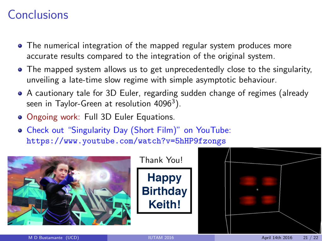
46. Conclusions The numerical integration of the mapped regular system produces more accurate results compared to the integration of the original system. The mapped system allows us to get unprecedentedly close to the singularity, unveiling a late-time slow regime with simple asymptotic behaviour. A cautionary tale for 3D Euler, regarding sudden change of regimes (already seen in Taylor-Green at resolution 40963 ). Ongoing work: Full 3D Euler Equations. M D Bustamante (UCD) IUTAM 2016 April 14th 2016 21 / 22
47. Conclusions The numerical integration of the mapped regular system produces more accurate results compared to the integration of the original system. The mapped system allows us to get unprecedentedly close to the singularity, unveiling a late-time slow regime with simple asymptotic behaviour. A cautionary tale for 3D Euler, regarding sudden change of regimes (already seen in Taylor-Green at resolution 40963 ). Ongoing work: Full 3D Euler Equations. Check out “Singularity Day (Short Film)” on YouTube: https://www.youtube.com/watch?v=5hHP9fzongs Thank You! M D Bustamante (UCD) IUTAM 2016 April 14th 2016 21 / 22 Happy Birthday Keith!
48. Further references (sample) High order pseudospectral calculations (with symmetries) [Brachet et al., JFM 130:411 (1983)] [Kerr, Phys. Fluids A 5:1725 (1993)] [Hou & Li, J. Nonlinear Sci. 16:639 (2006)] [Bustamante & Kerr, Physica D 237:1912 (2008)] Novel diagnostics (merging analyticity strip+BKM, Lagrangian element tracking) [Beale et al., Commun. Math. Phys 94:61 (1984)] [Frisch et al., Journal of Statistical Physics 113:761 (2003)] [Bustamante et al., Phys. Rev. E 86:066302 (2012)] [ Brachet et al., Phys. Rev. E 87:013110 (2013)] Spatial adaptivity (concentrate computations on localising structures) [Grafke et al., Physica D 237:1932 (2008)] ‘Engineered’ initial conditions [Lu and Doering, Indiana University Mathematics Journal 57:2693 (2008)] [Ayala & Protas, Physica D 240:1553 (2011)] Conditional regularity results (local geometric constraints on vorticity field) [Constantin et al., Comm. Partial Di↵erential Equations 21:559 (1996)] [Deng et al., Comm. Partial Di↵erential Equations 31:293 (2006)] Mapping to regular systems (3D Euler, 3D MHD, 2.5D Euler, etc.) [Bustamante, Physica D 240:1092 (2011)] [Mulungye, Lucas & Bustamante, J. Fluid Mech. 771:468 (2015)] [MLB J. Fluid Mech. 788:R3 (2016)] Symmetry plane models (2.5D) [Gibbon et al., Physica D 132:497 (1999)] [Ohkitani and Gibbon, Phys. Fluids 12:3181 (2000)] [Mulungye et al., op. cit.] M D Bustamante (UCD) IUTAM 2016 April 14th 2016 22 / 22