Multi-Armed Bandit Learning in IoT Networks: Decentralized Multi-Player Multi-Arm Bandits (16:9)

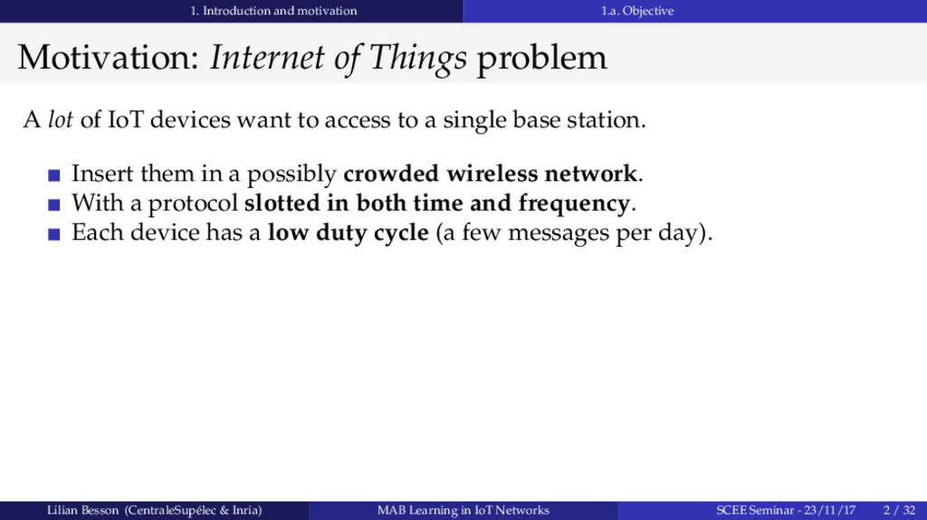
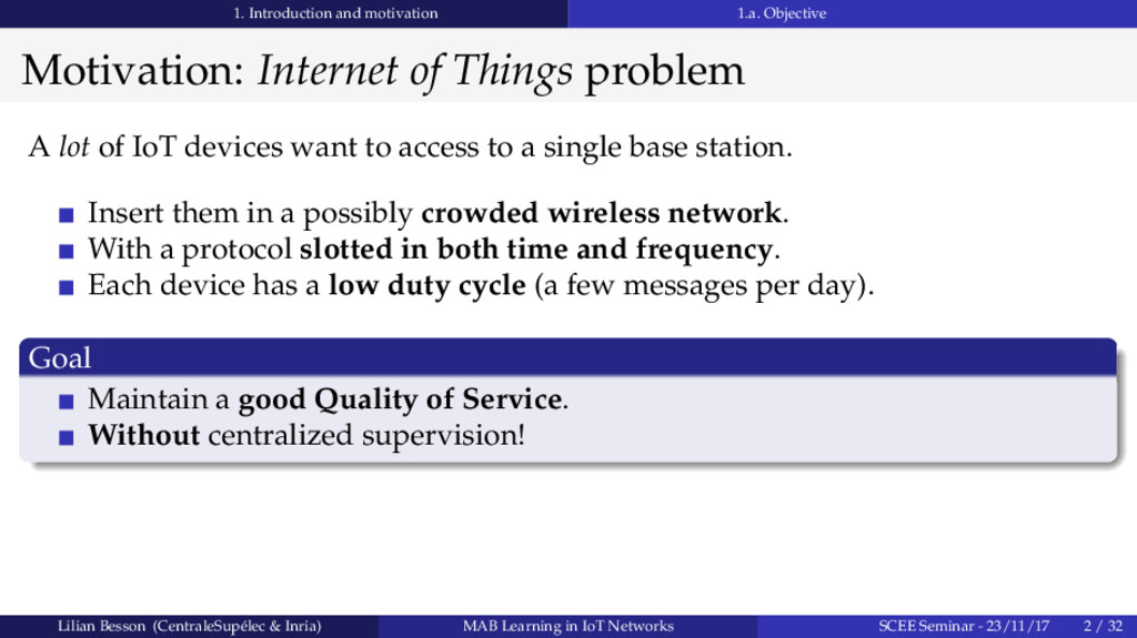
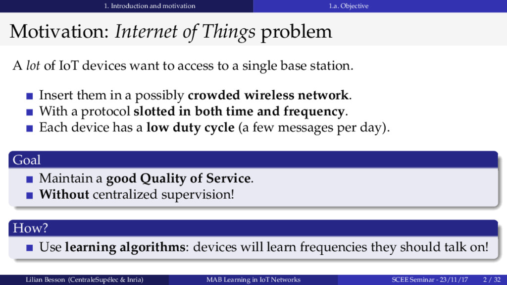
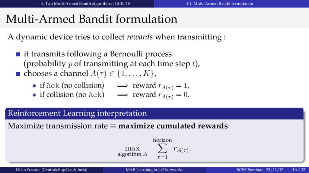
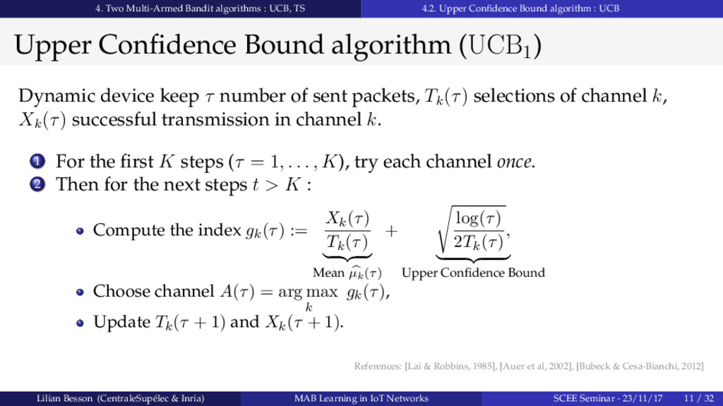
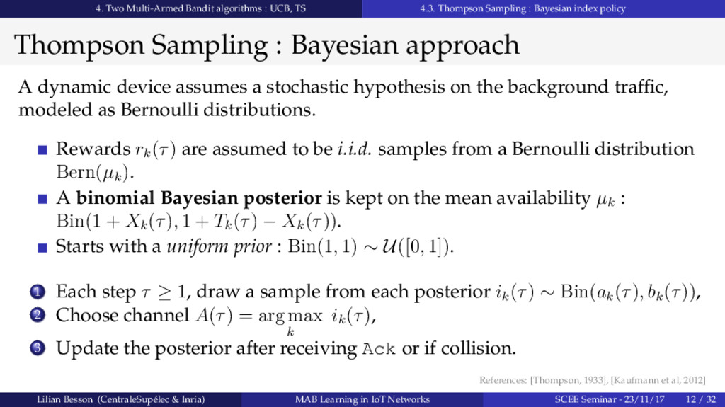
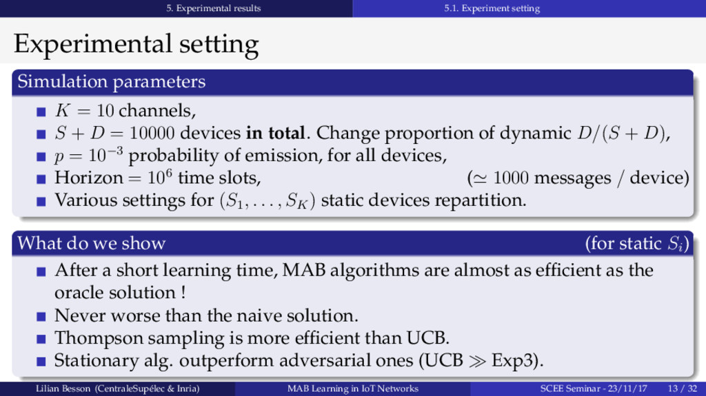
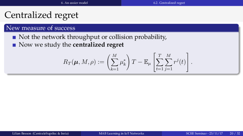
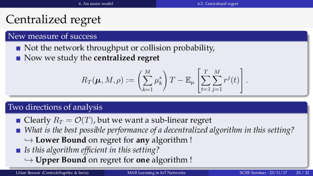
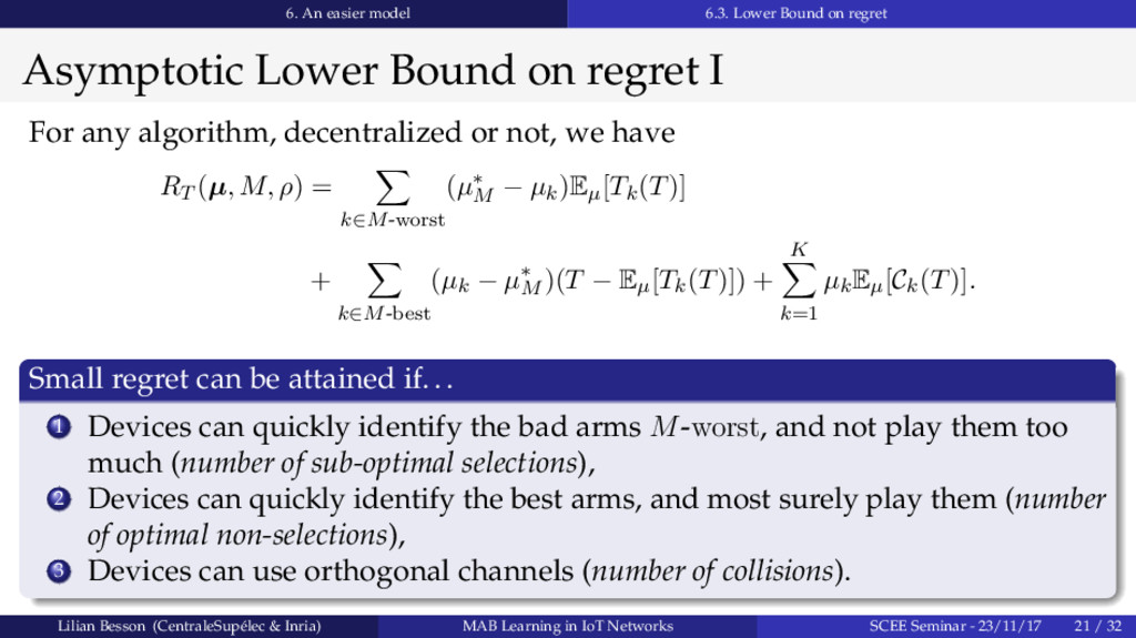
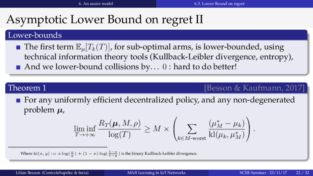
Setting up the future Internet of Things (IoT) networks will require to support more and more communicating devices. We prove that intelligent devices in unlicensed bands can use Multi-Armed Bandit (MAB) learning algorithms to improve resource exploitation. We evaluate the performance of two classical MAB learning algorithms, UCB1 and Thompson Sampling, to handle the decentralized decision-making of Spectrum Access, applied to IoT networks; as well as learning performance with a growing number of intelligent end-devices. We show that using learning algorithms does help to fit more devices in such networks, even when all end-devices are intelligent and are dynamically changing channel. In the studied scenario, stochastic MAB learning provides a up to 16% gain in term of successful transmission probabilities, and has near optimal performance even in non-stationary and non-i.i.d. settings with a majority of intelligent devices.

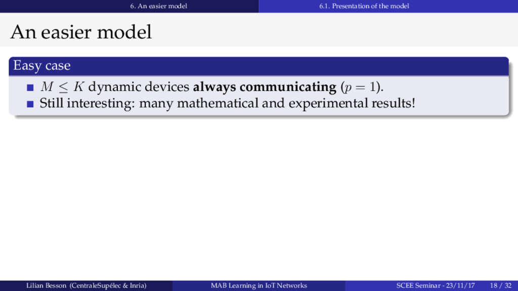
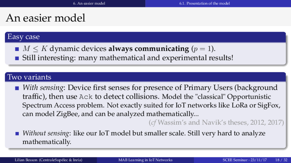
Additionally, I give insights on the latest theoretical results we obtained in the simplest case with let say 10 objects always communicating in at least 10 channels. Extending our results to the case of many objects communicating less frequently is significantly harder and will be dealt with during my 2nd year of PhD.

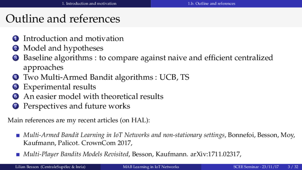
Main references are my recent articles (on HAL):

- Multi-Armed Bandit Learning in IoT Networks and non-stationary settings, Bonnefoi, Besson, Moy, Kaufmann, Palicot. CrownCom 2017. https://hal.inria.fr/hal-01575419
- Multi-Player Bandits Models Revisited, Besson, Kaufmann. arXiv:1711.02317. https://hal.inria.fr/hal-01629733

PDF: https://perso.crans.org/besson/publis/slides/2017_11__Presentation_Supelec_SCEE_Seminar/slides_169.pdf

Transcript

1. MAB Learning in IoT Networks Decentralized Multi-Player Multi-Arm Bandits Lilian Besson Advised by Christophe Moy Émilie Kaufmann PhD Student Team SCEE, IETR, CentraleSupélec, Rennes & Team SequeL, CRIStAL, Inria, Lille SCEE Seminar - 23 November 2017
2. 1. Introduction and motivation 1.a. Objective Motivation: Internet of Things problem A lot of IoT devices want to access to a single base station. Insert them in a possibly crowded wireless network. With a protocol slotted in both time and frequency. Each device has a low duty cycle (a few messages per day). Lilian Besson (CentraleSupélec & Inria) MAB Learning in IoT Networks SCEE Seminar - 23/11/17 2 / 32
3. 1. Introduction and motivation 1.a. Objective Motivation: Internet of Things problem A lot of IoT devices want to access to a single base station. Insert them in a possibly crowded wireless network. With a protocol slotted in both time and frequency. Each device has a low duty cycle (a few messages per day). Goal Maintain a good Quality of Service. Without centralized supervision! Lilian Besson (CentraleSupélec & Inria) MAB Learning in IoT Networks SCEE Seminar - 23/11/17 2 / 32
4. 1. Introduction and motivation 1.a. Objective Motivation: Internet of Things problem A lot of IoT devices want to access to a single base station. Insert them in a possibly crowded wireless network. With a protocol slotted in both time and frequency. Each device has a low duty cycle (a few messages per day). Goal Maintain a good Quality of Service. Without centralized supervision! How? Use learning algorithms: devices will learn frequencies they should talk on! Lilian Besson (CentraleSupélec & Inria) MAB Learning in IoT Networks SCEE Seminar - 23/11/17 2 / 32
5. 1. Introduction and motivation 1.b. Outline and references Outline and references 1 Introduction and motivation 2 Model and hypotheses 3 Baseline algorithms : to compare against naive and efficient centralized approaches 4 Two Multi-Armed Bandit algorithms : UCB, TS 5 Experimental results 6 An easier model with theoretical results 7 Perspectives and future works Main references are my recent articles (on HAL): Multi-Armed Bandit Learning in IoT Networks and non-stationary settings, Bonnefoi, Besson, Moy, Kaufmann, Palicot. CrownCom 2017, Multi-Player Bandits Models Revisited, Besson, Kaufmann. arXiv:1711.02317, Lilian Besson (CentraleSupélec & Inria) MAB Learning in IoT Networks SCEE Seminar - 23/11/17 3 / 32
6. 2. Model and hypotheses 2.a. First model First model Discrete time t ≥ 1 and K radio channels (e.g., 10) (known) Figure 1: Protocol in time and frequency, with an Acknowledgement. D dynamic devices try to access the network independently S = S1 + · · · + SK static devices occupy the network : S1 , . . . , SK in each channel (unknown) Lilian Besson (CentraleSupélec & Inria) MAB Learning in IoT Networks SCEE Seminar - 23/11/17 4 / 32
7. 2. Model and hypotheses 2.b. Hypotheses Hypotheses I Emission model Each device has the same low emission probability: each step, each device sends a packet with probability p. (this gives a duty cycle proportional to 1/p) Background traffic Each static device uses only one channel. Their repartition is fixed in time. =⇒ Background traffic, bothering the dynamic devices! Lilian Besson (CentraleSupélec & Inria) MAB Learning in IoT Networks SCEE Seminar - 23/11/17 5 / 32
8. 2. Model and hypotheses 2.b. Hypotheses Hypotheses II Dynamic radio reconfiguration Each dynamic device decides the channel it uses to send every packet. It has memory and computational capacity to implement simple decision algorithm. Problem Goal : minimize packet loss ratio (= maximize number of received Ack) in a finite-space discrete-time Decision Making Problem. Solution ? Multi-Armed Bandit algorithms, decentralized and used independently by each device. Lilian Besson (CentraleSupélec & Inria) MAB Learning in IoT Networks SCEE Seminar - 23/11/17 6 / 32
9. 3. Baseline algorithms 3.a. A naive strategy : uniformly random access A naive strategy : uniformly random access Uniformly random access: dynamic devices choose uniformly their channel in the pull of K channels. Natural strategy, dead simple to implement. Simple analysis, in term of successful transmission probability (for every message from dynamic devices) : P(success|sent) = K i=1 (1 − p/K)D−1 No other dynamic device × (1 − p)Si No static device × 1 K . Lilian Besson (CentraleSupélec & Inria) MAB Learning in IoT Networks SCEE Seminar - 23/11/17 7 / 32
10. 3. Baseline algorithms 3.a. A naive strategy : uniformly random access A naive strategy : uniformly random access Uniformly random access: dynamic devices choose uniformly their channel in the pull of K channels. Natural strategy, dead simple to implement. Simple analysis, in term of successful transmission probability (for every message from dynamic devices) : P(success|sent) = K i=1 (1 − p/K)D−1 No other dynamic device × (1 − p)Si No static device × 1 K . No learning Works fine only if all channels are similarly occupied, but it cannot learn to exploit the best (more free) channels. Lilian Besson (CentraleSupélec & Inria) MAB Learning in IoT Networks SCEE Seminar - 23/11/17 7 / 32
11. 3. Baseline algorithms 3.b. Optimal centralized strategy Optimal centralized strategy I If an oracle can decide to affect Di dynamic devices to channel i, the successful transmission probability is: P(success|sent) = K i=1 (1 − p)Di−1 Di−1 others × (1 − p)Si No static device × Di /D Sent in channel i . The oracle has to solve this optimization problem:    arg max D1,...,DK K i=1 Di(1 − p)Si +Di−1 such that K i=1 Di = D and Di ≥ 0, ∀1 ≤ i ≤ K. We solved this quasi-convex optimization problem with Lagrange multipliers, only numerically. Lilian Besson (CentraleSupélec & Inria) MAB Learning in IoT Networks SCEE Seminar - 23/11/17 8 / 32
12. 3. Baseline algorithms 3.b. Optimal centralized strategy Optimal centralized strategy II =⇒ Very good performance, maximizing the transmission rate of all the D dynamic devices But unrealistic But not achievable in practice: no centralized control and no oracle! Now let see realistic decentralized approaches ֒→ Machine Learning ? ֒→ Reinforcement Learning ? ֒→ Multi-Armed Bandit ! Lilian Besson (CentraleSupélec & Inria) MAB Learning in IoT Networks SCEE Seminar - 23/11/17 9 / 32
13. 4. Two Multi-Armed Bandit algorithms : UCB, TS 4.1. Multi-Armed Bandit formulation Multi-Armed Bandit formulation A dynamic device tries to collect rewards when transmitting : it transmits following a Bernoulli process (probability p of transmitting at each time step t), chooses a channel A(τ) ∈ {1, . . . , K}, if Ack (no collision) =⇒ reward rA(τ) = 1, if collision (no Ack) =⇒ reward rA(τ) = 0. Reinforcement Learning interpretation Maximize transmission rate ≡ maximize cumulated rewards max algorithm A horizon τ=1 rA(τ) . Lilian Besson (CentraleSupélec & Inria) MAB Learning in IoT Networks SCEE Seminar - 23/11/17 10 / 32
14. 4. Two Multi-Armed Bandit algorithms : UCB, TS 4.2. Upper Confidence Bound algorithm : UCB Upper Confidence Bound algorithm (UCB1 ) Dynamic device keep τ number of sent packets, Tk (τ) selections of channel k, Xk (τ) successful transmission in channel k. 1 For the first K steps (τ = 1, . . . , K), try each channel once. 2 Then for the next steps t > K : Compute the index gk(τ) := Xk(τ) Tk(τ) Mean µk (τ) + log(τ) 2Tk(τ) , Upper Confidence Bound Choose channel A(τ) = arg max k gk(τ), Update Tk(τ + 1) and Xk(τ + 1). References: [Lai & Robbins, 1985], [Auer et al, 2002], [Bubeck & Cesa-Bianchi, 2012] Lilian Besson (CentraleSupélec & Inria) MAB Learning in IoT Networks SCEE Seminar - 23/11/17 11 / 32
15. 4. Two Multi-Armed Bandit algorithms : UCB, TS 4.3. Thompson Sampling : Bayesian index policy Thompson Sampling : Bayesian approach A dynamic device assumes a stochastic hypothesis on the background traffic, modeled as Bernoulli distributions. Rewards rk (τ) are assumed to be i.i.d. samples from a Bernoulli distribution Bern(µk ). A binomial Bayesian posterior is kept on the mean availability µk : Bin(1 + Xk (τ), 1 + Tk (τ) − Xk (τ)). Starts with a uniform prior : Bin(1, 1) ∼ U([0, 1]). 1 Each step τ ≥ 1, draw a sample from each posterior ik (τ) ∼ Bin(ak (τ), bk (τ)), 2 Choose channel A(τ) = arg max k ik (τ), 3 Update the posterior after receiving Ack or if collision. References: [Thompson, 1933], [Kaufmann et al, 2012] Lilian Besson (CentraleSupélec & Inria) MAB Learning in IoT Networks SCEE Seminar - 23/11/17 12 / 32
16. 5. Experimental results 5.1. Experiment setting Experimental setting Simulation parameters K = 10 channels, S + D = 10000 devices in total. Change proportion of dynamic D/(S + D), p = 10−3 probability of emission, for all devices, Horizon = 106 time slots, (≃ 1000 messages / device) Various settings for (S1 , . . . , SK ) static devices repartition. What do we show (for static Si ) After a short learning time, MAB algorithms are almost as efficient as the oracle solution ! Never worse than the naive solution. Thompson sampling is more efficient than UCB. Stationary alg. outperform adversarial ones (UCB ≫ Exp3). Lilian Besson (CentraleSupélec & Inria) MAB Learning in IoT Networks SCEE Seminar - 23/11/17 13 / 32
17. 5. Experimental results 5.2. First result: 10% 10% of dynamic devices Number of slots ×105 2 4 6 8 10 Successful transmission rate 0.82 0.83 0.84 0.85 0.86 0.87 0.88 0.89 0.9 0.91 UCB Thompson-sampling Optimal Good sub-optimal Random Figure 2: 10% of dynamic devices. 7% of gain. Lilian Besson (CentraleSupélec & Inria) MAB Learning in IoT Networks SCEE Seminar - 23/11/17 14 / 32
18. 5. Experimental results 5.2. First result: 20% 30% of dynamic devices Number of slots ×105 2 4 6 8 10 Successful transmission rate 0.81 0.815 0.82 0.825 0.83 0.835 0.84 0.845 0.85 0.855 0.86 UCB Thompson-sampling Optimal Good sub-optimal Random Figure 3: 30% of dynamic devices. 3% of gain but not much is possible. Lilian Besson (CentraleSupélec & Inria) MAB Learning in IoT Networks SCEE Seminar - 23/11/17 15 / 32
19. 5. Experimental results 5.3. Growing proportion of devices dynamic devices Dependence on D/(S + D) Proportion of dynamic devices (%) 0.1 0.2 0.3 0.4 0.5 0.6 0.7 0.8 0.9 Gain compared to random channel selection -0.02 0 0.02 0.04 0.06 0.08 0.1 0.12 0.14 0.16 Optimal strategy UCB 1 , α=0.5 Thomson-sampling Figure 4: Almost optimal, for any proportion of dynamic devices, after a short learning time. Up-to 16% gain over the naive approach! Lilian Besson (CentraleSupélec & Inria) MAB Learning in IoT Networks SCEE Seminar - 23/11/17 16 / 32
20. 6. An easier model Section 6 A brief presentation of a different approach... Theoretical results for an easier model Lilian Besson (CentraleSupélec & Inria) MAB Learning in IoT Networks SCEE Seminar - 23/11/17 17 / 32
21. 6. An easier model 6.1. Presentation of the model An easier model Easy case M ≤ K dynamic devices always communicating (p = 1). Still interesting: many mathematical and experimental results! Lilian Besson (CentraleSupélec & Inria) MAB Learning in IoT Networks SCEE Seminar - 23/11/17 18 / 32
22. 6. An easier model 6.1. Presentation of the model An easier model Easy case M ≤ K dynamic devices always communicating (p = 1). Still interesting: many mathematical and experimental results! Two variants With sensing: Device first senses for presence of Primary Users (background traffic), then use Ack to detect collisions. Model the "classical" Opportunistic Spectrum Access problem. Not exactly suited for IoT networks like LoRa or SigFox, can model ZigBee, and can be analyzed mathematically... (cf Wassim’s and Navik’s theses, 2012, 2017) Without sensing: like our IoT model but smaller scale. Still very hard to analyze mathematically. Lilian Besson (CentraleSupélec & Inria) MAB Learning in IoT Networks SCEE Seminar - 23/11/17 18 / 32
23. 6. An easier model 6.2. Notations Notations for this second model Notations K channels, modeled as Bernoulli (0/1) distributions of mean µk = background traffic from Primary Users, M devices use channel Aj(t) ∈ {1, . . . , K} at each time step, Reward: rj(t) := YAj(t),t × ✶(Cj(t)) = ✶(uplink & Ack) with sensing information Yk,t ∼ Bern(µk), collision for device j Cj(t) = ✶(alone on arm Aj(t)). Lilian Besson (CentraleSupélec & Inria) MAB Learning in IoT Networks SCEE Seminar - 23/11/17 19 / 32
24. 6. An easier model 6.2. Notations Notations for this second model Notations K channels, modeled as Bernoulli (0/1) distributions of mean µk = background traffic from Primary Users, M devices use channel Aj(t) ∈ {1, . . . , K} at each time step, Reward: rj(t) := YAj(t),t × ✶(Cj(t)) = ✶(uplink & Ack) with sensing information Yk,t ∼ Bern(µk), collision for device j Cj(t) = ✶(alone on arm Aj(t)). Goal : decentralized reinforcement learning optimization! Each player wants to maximize its cumulated reward, With no central control, and no exchange of information, Only possible if : each player converges to one of the M best arms, orthogonally (without collisions) Lilian Besson (CentraleSupélec & Inria) MAB Learning in IoT Networks SCEE Seminar - 23/11/17 19 / 32
25. 6. An easier model 6.2. Centralized regret Centralized regret New measure of success Not the network throughput or collision probability, Now we study the centralized regret RT (µ, M, ρ) := M k=1 µ∗ k T − Eµ   T t=1 M j=1 rj(t)   . Lilian Besson (CentraleSupélec & Inria) MAB Learning in IoT Networks SCEE Seminar - 23/11/17 20 / 32
26. 6. An easier model 6.2. Centralized regret Centralized regret New measure of success Not the network throughput or collision probability, Now we study the centralized regret RT (µ, M, ρ) := M k=1 µ∗ k T − Eµ   T t=1 M j=1 rj(t)   . Two directions of analysis Clearly RT = O(T), but we want a sub-linear regret What is the best possible performance of a decentralized algorithm in this setting? ֒→ Lower Bound on regret for any algorithm ! Is this algorithm efficient in this setting? ֒→ Upper Bound on regret for one algorithm ! Lilian Besson (CentraleSupélec & Inria) MAB Learning in IoT Networks SCEE Seminar - 23/11/17 20 / 32
27. 6. An easier model 6.3. Lower Bound on regret Asymptotic Lower Bound on regret I For any algorithm, decentralized or not, we have RT (µ, M, ρ) = k∈M-worst (µ∗ M − µk)Eµ[Tk(T)] + k∈M-best (µk − µ∗ M )(T − Eµ[Tk(T)]) + K k=1 µkEµ[Ck(T)]. Small regret can be attained if. .. 1 Devices can quickly identify the bad arms M-worst, and not play them too much (number of sub-optimal selections), 2 Devices can quickly identify the best arms, and most surely play them (number of optimal non-selections), 3 Devices can use orthogonal channels (number of collisions). Lilian Besson (CentraleSupélec & Inria) MAB Learning in IoT Networks SCEE Seminar - 23/11/17 21 / 32
28. 6. An easier model 6.3. Lower Bound on regret Asymptotic Lower Bound on regret II Lower-bounds The first term Eµ [Tk (T)], for sub-optimal arms, is lower-bounded, using technical information theory tools (Kullback-Leibler divergence, entropy), And we lower-bound collisions by... 0 : hard to do better! Theorem 1 [Besson & Kaufmann, 2017] For any uniformly efficient decentralized policy, and any non-degenerated problem µ, lim inf T→+∞ RT (µ, M, ρ) log(T) ≥ M ×   k∈M-worst (µ∗ M − µk ) kl(µk , µ∗ M )   . Where kl(x, y) := x log( x y ) + (1 − x) log( 1−x 1−y ) is the binary Kullback-Leibler divergence. Lilian Besson (CentraleSupélec & Inria) MAB Learning in IoT Networks SCEE Seminar - 23/11/17 22 / 32
29. Illustration of the Lower Bound on regret 0 2000 4000 6000 8000 10000 Time steps t = 1. . T , horizon T = 10000 , 6 players: 6 × RhoRand-KLUCB 0 500 1000 1500 2000 2500 Cumulative centralized regret 1000 [R t ] Multi-players M = 6 : Cumulated centralized regret, averaged 1000 times 9 arms: [B(0.1), B(0.2), B(0.3), B(0.4) ∗ , B(0.5) ∗ , B(0.6) ∗ , B(0.7) ∗ , B(0.8) ∗ , B(0.9) ∗ ] Cumulated centralized regret (a) term: Pulls of 3 suboptimal arms (lower-bounded) (b) term: Non-pulls of 6 optimal arms (c) term: Weighted count of collisions Our lower-bound = 48.8 log(t) Anandkumar et al.'s lower-bound = 15 log(t) Centralized lower-bound = 8.14 log(t) Figure 5: Any such lower-bound is very asymptotic, usually not satisfied for small horizons. We can see the importance of the collisions!
30. 6. An easier model 6.4. Algorithms Algorithms for this easier model Building blocks : separate the two aspects 1 MAB policy to learn the best arms (use sensing YAj(t),t ), 2 Orthogonalization scheme to avoid collisions (use Cj(t)). Lilian Besson (CentraleSupélec & Inria) MAB Learning in IoT Networks SCEE Seminar - 23/11/17 24 / 32
31. 6. An easier model 6.4. Algorithms Algorithms for this easier model Building blocks : separate the two aspects 1 MAB policy to learn the best arms (use sensing YAj(t),t ), 2 Orthogonalization scheme to avoid collisions (use Cj(t)). Many different proposals for decentralized learning policies Recent: MEGA and Musical Chair, [Avner & Mannor, 2015], [Shamir et al, 2016] State-of-the-art: RhoRand policy and variants, [Anandkumar et al, 2011] Our proposals: [Besson & Kaufmann, 2017] With sensing: RandTopM and MCTopM are sort of mixes between RhoRand and Musical Chair, using UCB indexes or more efficient index policy (kl-UCB), Without sensing: Selfish use a UCB index directly on the reward rj(t) : like the first IoT model ! Lilian Besson (CentraleSupélec & Inria) MAB Learning in IoT Networks SCEE Seminar - 23/11/17 24 / 32
32. Illustration of different algorithms 0 1000 2000 3000 4000 5000 Time steps t = 1. . T , horizon T = 5000 , 0 500 1000 1500 2000 2500 3000 3500 Cumulative centralized regret 6 k = 1 µ ∗ k t − 9 k = 1 µ k 500 [T k (t)] Multi-players M = 6 : Cumulated centralized regret, averaged 500 times 9 arms: Bayesian MAB, Bernoulli with means on [0, 1] 6 × RandTopM-KLUCB 6 × MCTopM-KLUCB 6 × Selfish-KLUCB 6 × RhoRand-KLUCB Figure 6: Regret, M = 6 players, K = 9 arms, horizon T = 5000, against 500 problems µ uniformly sampled in [0, 1]K. RhoRand < RandTopM < Selfish < MCTopM in most cases.
33. 6. An easier model 6.5. Regret upper-bound Regret upper-bound for MCTopM-kl-UCB Theorem 2 [Besson & Kaufmann, 2017] If all M players use MCTopM-kl-UCB, for any non-degenerated problem µ, RT (µ, M, ρ) ≤ GM,µ log(T) + o(log T) . Remarks Hard to prove, we had to carefully design the MCTopM algorithm to conclude, For the suboptimal selections, we match our lower-bound ! We also minimize the number of channel switching: interesting as it costs energy, Not yet possible to know what is the best possible control of collisions... Lilian Besson (CentraleSupélec & Inria) MAB Learning in IoT Networks SCEE Seminar - 23/11/17 26 / 32
34. 6. An easier model 6.6. Problems with Selfish In this model The Selfish decentralized approach = device don’t use sensing, just learn on the receive acknowledgement, Like our first IoT model, It works fine in practice! Except... when it fails drastically! In small problems with M and K = 2 or 3, we found small probability of failures (i.e., linear regret), and this prevents from having a generic upper-bound on regret for Selfish. Sadly... Lilian Besson (CentraleSupélec & Inria) MAB Learning in IoT Networks SCEE Seminar - 23/11/17 27 / 32
35. Illustration of failing cases for Selfish 10 15 20 25 30 35 0 20 40 60 80 100 120 6 5 4 2 × RandTopM-KLUCB 0 1000 2000 3000 4000 5000 6000 7000 0 200 400 600 800 1000 17 2 × Selfish-KLUCB 10 15 20 25 30 35 40 0 20 40 60 80 100 120 140 2 1 2 1 2 × MCTopM-KLUCB 10 20 30 40 50 60 0 20 40 60 80 100 120 140 160 2 2 2 × RhoRand-KLUCB 0.0 0.2 0.4 0.6 0.8 1.0 Regret value R T at the end of simulation, for T = 5000 0.0 0.2 0.4 0.6 0.8 1.0 Number of observations, 1000 repetitions Histogram of regrets for different multi-players bandit algorithms 3 arms: [B(0.1), B(0.5) ∗ , B(0.9) ∗ ] Figure 7: Histograms of regret for M = 2 players, K = 3 arms, horizon T = 5000, 1000 repetitions and µ = [0.1, 0.5, 0.9] (different scales). Selfish have a small probability of failure (17 cases of RT ≥ T, out of 1000). The regret for the other algorithms is very small for such “easy” problem.
36. 7. Perspectives and future work 7.1. Perspectives Perspectives Theoretical results MAB algorithms have guarantees for i.i.d. settings, But here the collisions cancel the i.i.d. hypothesis, Not easy to obtain guarantees in this mixed setting (i.i.d. emissions process, “game theoretic” collisions). For OSA devices (always emitting), we obtained strong theoretical results, But harder for IoT devices with low duty-cycle. .. Real-world experimental validation ? Radio experiments will help to validate this. Hard ! Lilian Besson (CentraleSupélec & Inria) MAB Learning in IoT Networks SCEE Seminar - 23/11/17 29 / 32
37. 7. Perspectives and future work 7.2. Future work Other directions of future work More realistic emission model: maybe driven by number of packets in a whole day, instead of emission probability. Validate this on a larger experimental scale. Extend the theoretical analysis to the large-scale IoT model, first with sensing (e.g., models ZigBee networks), then without sensing (e.g., LoRaWAN networks). And also conclude the Multi-Player OSA analysis (remove hypothesis that objects know M, allow arrival/departure of objects, non-stationarity of background traffic etc) Lilian Besson (CentraleSupélec & Inria) MAB Learning in IoT Networks SCEE Seminar - 23/11/17 30 / 32
38. 7. Conclusion 7.3 Thanks! Conclusion I We showed Simple Multi-Armed Bandit algorithms, used in a Selfish approach by IoT devices in a crowded network, help to quickly learn the best possible repartition of dynamic devices in a fully decentralized and automatic way, For devices with sensing, smarter algorithms can be designed, and analyze carefully. Empirically, even if the collisions break the i.i.d hypothesis, stationary MAB algorithms (UCB, TS, kl-UCB) outperform more generic algorithms (adversarial, like Exp3). Lilian Besson (CentraleSupélec & Inria) MAB Learning in IoT Networks SCEE Seminar - 23/11/17 31 / 32
39. 7. Conclusion 7.3 Thanks! Conclusion II But more work is still needed. .. Theoretical guarantees are still missing for the IoT model, and can be improved (slightly) for the OSA model. Maybe study other emission models. Implement this on real-world radio devices (TestBed). Thanks! Any question? Lilian Besson (CentraleSupélec & Inria) MAB Learning in IoT Networks SCEE Seminar - 23/11/17 32 / 32