r e I n c . F M E T u t o r i a l Contents iii Contents Chapter 1 Getting Started .................................................................................................................................. 1 Installing FME.............................................................................................................................................. 1 Licensing FME .............................................................................................................................................. 1 Installing the FME Sample Dataset.................................................................................................................. 1 Getting help ................................................................................................................................................ 1 Chapter 2 Viewing Data – FME Universal Viewer ................................................................................................ 2 In this chapter ............................................................................................................................................. 2 Objective .................................................................................................................................................... 2 Viewing data ............................................................................................................................................... 2 Viewing geometry and attributes ............................................................................................................ 3 Getting coordinate system information .................................................................................................... 4 Filtering features .................................................................................................................................. 4 Overlaying data in different formats................................................................................................................ 5 Exporting data from the Viewer ...................................................................................................................... 8 Chapter 3 Quick Translations – FME Universal Translator ................................................................................ 11 In this chapter ............................................................................................................................................11 Objective ...................................................................................................................................................11 Automating translations ...............................................................................................................................12 Processing basic features..............................................................................................................................13 Reprojecting data........................................................................................................................................15
r e I n c . F M E T u t o r i a l Contents iv Chapter 4 Custom Translations – FME Workbench............................................................................................ 18 In this chapter ............................................................................................................................................18 Objective ...................................................................................................................................................18 Creating a workspace...................................................................................................................................19 Using transformers......................................................................................................................................21 Creating custom formats ..............................................................................................................................35 Saving the workspace as a custom format...............................................................................................35 Associating the custom format with a different file extension .....................................................................36 Using the custom format to view data ....................................................................................................37 Working with custom transformers.................................................................................................................39 Creating custom transformers ...............................................................................................................39 Distributing custom transformers...........................................................................................................42 Appendix A Getting Started with Workbench ................................................................................................... 44 Workbench interface....................................................................................................................................44 Menu bar and Toolbar ..................................................................................................................................44 Color definitions ..................................................................................................................................46 Quick changes ............................................................................................................................................47 Renaming attributes ............................................................................................................................47 Creating new attributes ........................................................................................................................47 Editing existing attributes .....................................................................................................................47 Inserting transformer connections..........................................................................................................48 Inserting vertices on links.....................................................................................................................49
r e I n c . F M E T u t o r i a l Chapter 1: Getting Started 1 Chapter 1 Getting Started Installing FME The FME installer is a single application. There is only one installer for all FME license levels. 1. FME requires administrative privileges to install. This may require assistance from your system administrator. 2. Double-click setup.exe. 3. Answer the questions asked by the Installation Wizard. Licensing FME To license FME, run the FME Licensing Wizard available under Start > Program Files > FME and answer the questions asked by the wizard. Note: This Tutorial is designed specifically for use with FME 2009. Some of the functionality described may not be available when used in conjunction with older FME versions. Installing the FME Sample Dataset Download the FME Sample Dataset from www.safe.com/support/onlinelearning/fmesampledata.php and extract the contents to C:\FMEData. Note: You can access this Tutorial at www.safe.com/tutorial as well. Getting help FME products include extensive, context-sensitive help. If you require assistance with a tool or format, select the item and press F1 to open the help system. If you have questions regarding licensing or installation, please e-mail [email protected].
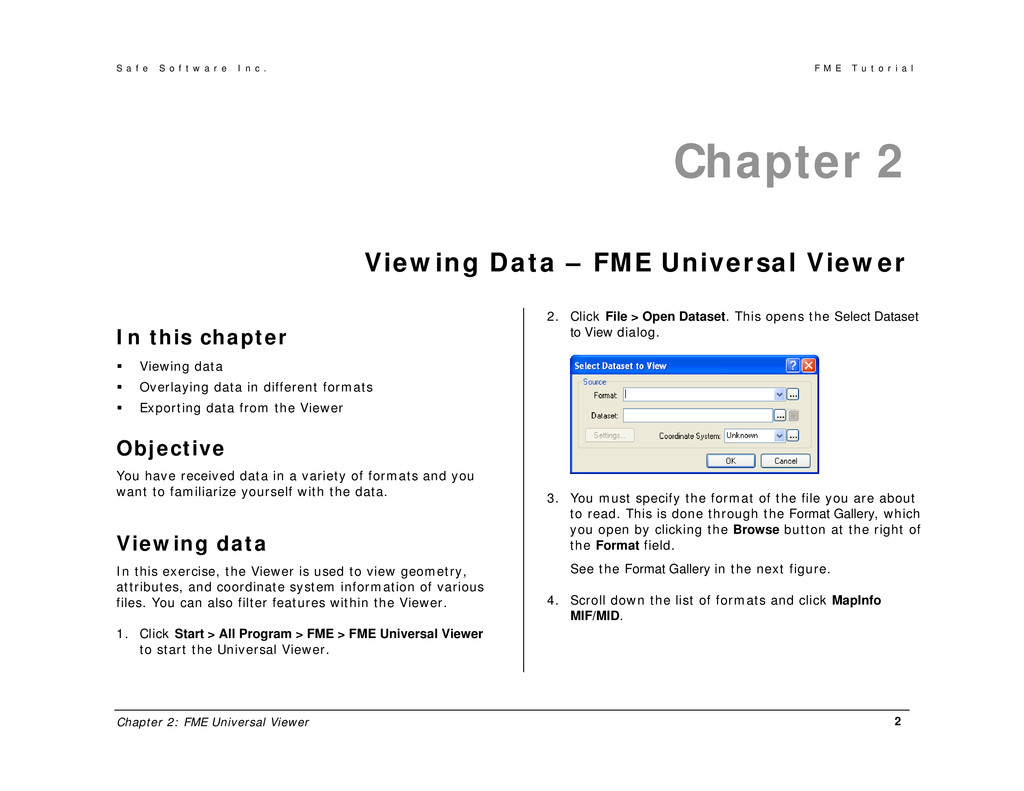
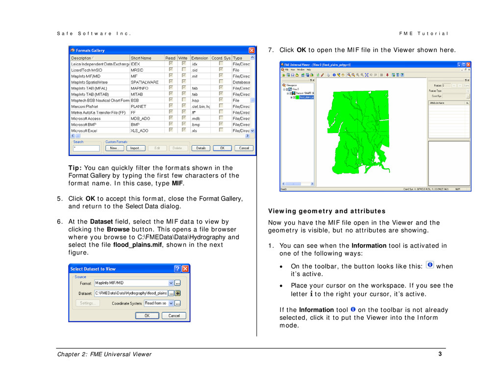
r e I n c . F M E T u t o r i a l Chapter 2: FME Universal Viewer 2 Chapter 2 Viewing Data – FME Universal Viewer In this chapter Viewing data Overlaying data in different formats Exporting data from the Viewer Objective You have received data in a variety of formats and you want to familiarize yourself with the data. Viewing data In this exercise, the Viewer is used to view geometry, attributes, and coordinate system information of various files. You can also filter features within the Viewer. 1. Click Start > All Program > FME > FME Universal Viewer to start the Universal Viewer. 2. Click File > Open Dataset. This opens the Select Dataset to View dialog. 3. You must specify the format of the file you are about to read. This is done through the Format Gallery, which you open by clicking the Browse button at the right of the Format field. See the Format Gallery in the next figure. 4. Scroll down the list of formats and click MapInfo MIF/MID.
r e I n c . F M E T u t o r i a l Chapter 2: FME Universal Viewer 3 Tip: You can quickly filter the formats shown in the Format Gallery by typing the first few characters of the format name. In this case, type MIF. 5. Click OK to accept this format, close the Format Gallery, and return to the Select Data dialog. 6. At the Dataset field, select the MIF data to view by clicking the Browse button. This opens a file browser where you browse to C:\FMEData\Data\Hydrography and select the file flood_plains.mif, shown in the next figure. 7. Click OK to open the MIF file in the Viewer shown here. Viewing geometry and attributes Now you have the MIF file open in the Viewer and the geometry is visible, but no attributes are showing. 1. You can see when the Information tool is activated in one of the following ways: • On the toolbar, the button looks like this: when it’s active. • Place your cursor on the workspace. If you see the letter i to the right your cursor, it’s active. If the Information tool on the toolbar is not already selected, click it to put the Viewer into the Inform mode.
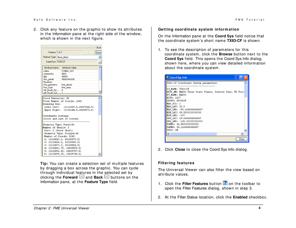
r e I n c . F M E T u t o r i a l Chapter 2: FME Universal Viewer 4 2. Click any feature on the graphic to show its attributes in the Information pane at the right side of the window, which is shown in the next figure. Tip: You can create a selection set of multiple features by dragging a box across the graphic. You can cycle through individual features in the selected set by clicking the Forward and Back buttons on the Information pane, at the Feature Type field. Getting coordinate system information On the Information pane at the Coord Sys field notice that the coordinate system’s short name TX83-CF is shown. 1. To see the description of parameters for this coordinate system, click the Browse button next to the Coord Sys field. This opens the Coord Sys Info dialog, shown here, where you can view detailed information about the coordinate system. 2. Click Close to close the Coord Sys Info dialog. Filtering features The Universal Viewer can also filter the view based on attribute values. 1. Click the Filter Features button on the toolbar to open the Filter Features dialog, shown in step 3. 2. At the Filter Status location, click the Enabled checkbox.
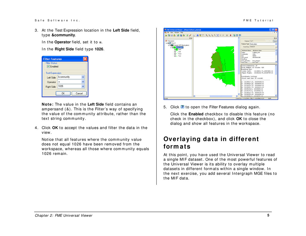
r e I n c . F M E T u t o r i a l Chapter 2: FME Universal Viewer 5 3. At the Test Expression location in the Left Side field, type &community. In the Operator field, set it to =. In the Right Side field type 1026. Note: The value in the Left Side field contains an ampersand (&). This is the Filter’s way of specifying the value of the community attribute, rather than the text string community. 4. Click OK to accept the values and filter the data in the view. Notice that all features where the community value does not equal 1026 have been removed from the workspace, whereas all those where community equals 1026 remain. 5. Click to open the Filter Features dialog again. Click the Enabled checkbox to disable this feature (no check in the checkbox), and click OK to close the dialog and show all features in the workspace. Overlaying data in different formats At this point, you have used the Universal Viewer to read a single MIF dataset. One of the most powerful features of the Universal Viewer is its ability to overlay multiple datasets in different formats within a single window. In the next exercise, you add several Intergraph MGE files to the MIF data.
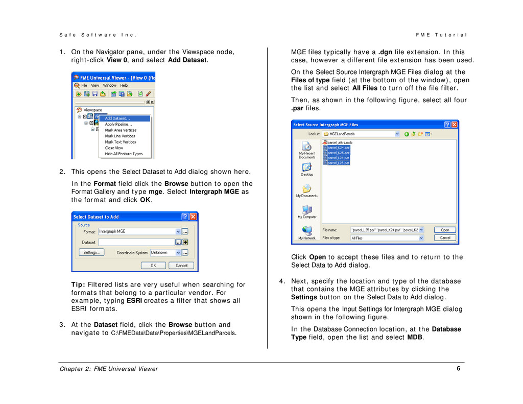
r e I n c . F M E T u t o r i a l Chapter 2: FME Universal Viewer 6 1. On the Navigator pane, under the Viewspace node, right-click View 0, and select Add Dataset. 2. This opens the Select Dataset to Add dialog shown here. In the Format field click the Browse button to open the Format Gallery and type mge. Select Intergraph MGE as the format and click OK. Tip: Filtered lists are very useful when searching for formats that belong to a particular vendor. For example, typing ESRI creates a filter that shows all ESRI formats. 3. At the Dataset field, click the Browse button and navigate to C:\FMEData\Data\Properties\MGELandParcels. MGE files typically have a .dgn file extension. In this case, however a different file extension has been used. On the Select Source Intergraph MGE Files dialog at the Files of type field (at the bottom of the window), open the list and select All Files to turn off the file filter. Then, as shown in the following figure, select all four .par files. Click Open to accept these files and to return to the Select Data to Add dialog. 4. Next, specify the location and type of the database that contains the MGE attributes by clicking the Settings button on the Select Data to Add dialog. This opens the Input Settings for Intergraph MGE dialog shown in the following figure. In the Database Connection location, at the Database Type field, open the list and select MDB.
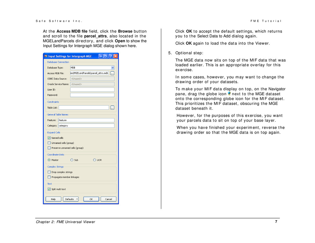
r e I n c . F M E T u t o r i a l Chapter 2: FME Universal Viewer 7 At the Access MDB file field, click the Browse button and scroll to the file parcel_attrs, also located in the MGELandParcels directory, and click Open to show the Input Settings for Intergraph MGE dialog shown here. Click OK to accept the default settings, which returns you to the Select Data to Add dialog again. Click OK again to load the data into the Viewer. 5. Optional step: The MGE data now sits on top of the MIF data that was loaded earlier. This is an appropriate overlay for this exercise. In some cases, however, you may want to change the drawing order of your datasets. To make your MIF data display on top, on the Navigator pane, drag the globe icon next to the MGE dataset onto the corresponding globe icon for the MIF dataset. This prioritizes the MIF dataset, obscuring the MGE dataset beneath it. However, for the purposes of this exercise, you want your parcels data to sit on top of your base layer. When you have finished your experiment, reverse the drawing order so that the MGE data is on top again.
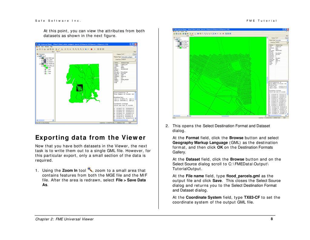
r e I n c . F M E T u t o r i a l Chapter 2: FME Universal Viewer 8 At this point, you can view the attributes from both datasets as shown in the next figure. Exporting data from the Viewer Now that you have both datasets in the Viewer, the next task is to write them out to a single GML file. However, for this particular export, only a small section of the data is required. 1. Using the Zoom In tool , zoom to a small area that contains features from both the MGE file and the MIF file. After the area is redrawn, select File > Save Data As. 2. This opens the Select Destination Format and Dataset dialog. At the Format field, click the Browse button and select Geography Markup Language (GML) as the destination format, and then click OK on the Destination Formats Gallery. At the Dataset field, click the Browse button and on the Select Source dialog scroll to C:\FMEData\Output\ TutorialOutput. At the File name field, type flood_parcels.gml as the output file and click Save. This closes the Select Source dialog and returns you to the Select Destination Format and Dataset dialog. At the Coordinate System field, type TX83-CF to set the coordinate system of the output GML file.
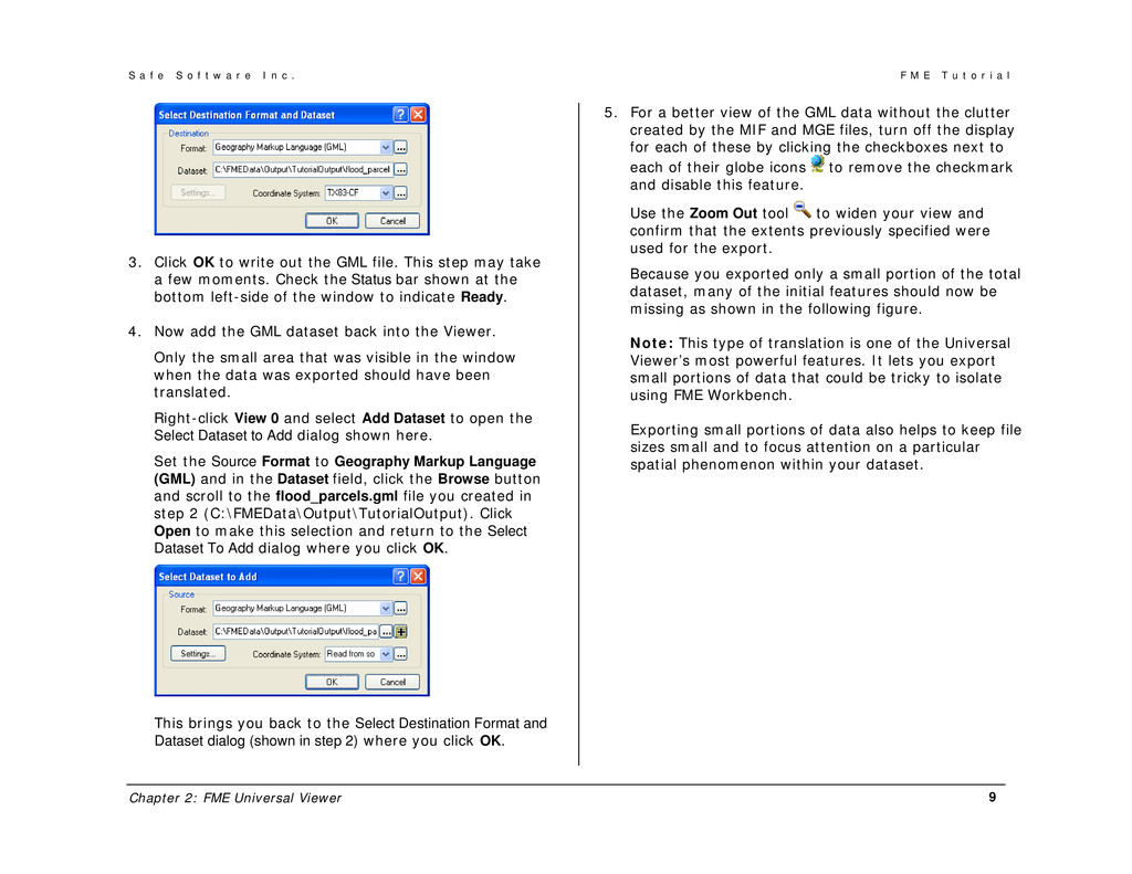
r e I n c . F M E T u t o r i a l Chapter 2: FME Universal Viewer 9 3. Click OK to write out the GML file. This step may take a few moments. Check the Status bar shown at the bottom left-side of the window to indicate Ready. 4. Now add the GML dataset back into the Viewer. Only the small area that was visible in the window when the data was exported should have been translated. Right-click View 0 and select Add Dataset to open the Select Dataset to Add dialog shown here. Set the Source Format to Geography Markup Language (GML) and in the Dataset field, click the Browse button and scroll to the flood_parcels.gml file you created in step 2 (C:\FMEData\Output\TutorialOutput). Click Open to make this selection and return to the Select Dataset To Add dialog where you click OK. This brings you back to the Select Destination Format and Dataset dialog (shown in step 2) where you click OK. 5. For a better view of the GML data without the clutter created by the MIF and MGE files, turn off the display for each of these by clicking the checkboxes next to each of their globe icons to remove the checkmark and disable this feature. Use the Zoom Out tool to widen your view and confirm that the extents previously specified were used for the export. Because you exported only a small portion of the total dataset, many of the initial features should now be missing as shown in the following figure. Note: This type of translation is one of the Universal Viewer’s most powerful features. It lets you export small portions of data that could be tricky to isolate using FME Workbench. Exporting small portions of data also helps to keep file sizes small and to focus attention on a particular spatial phenomenon within your dataset.
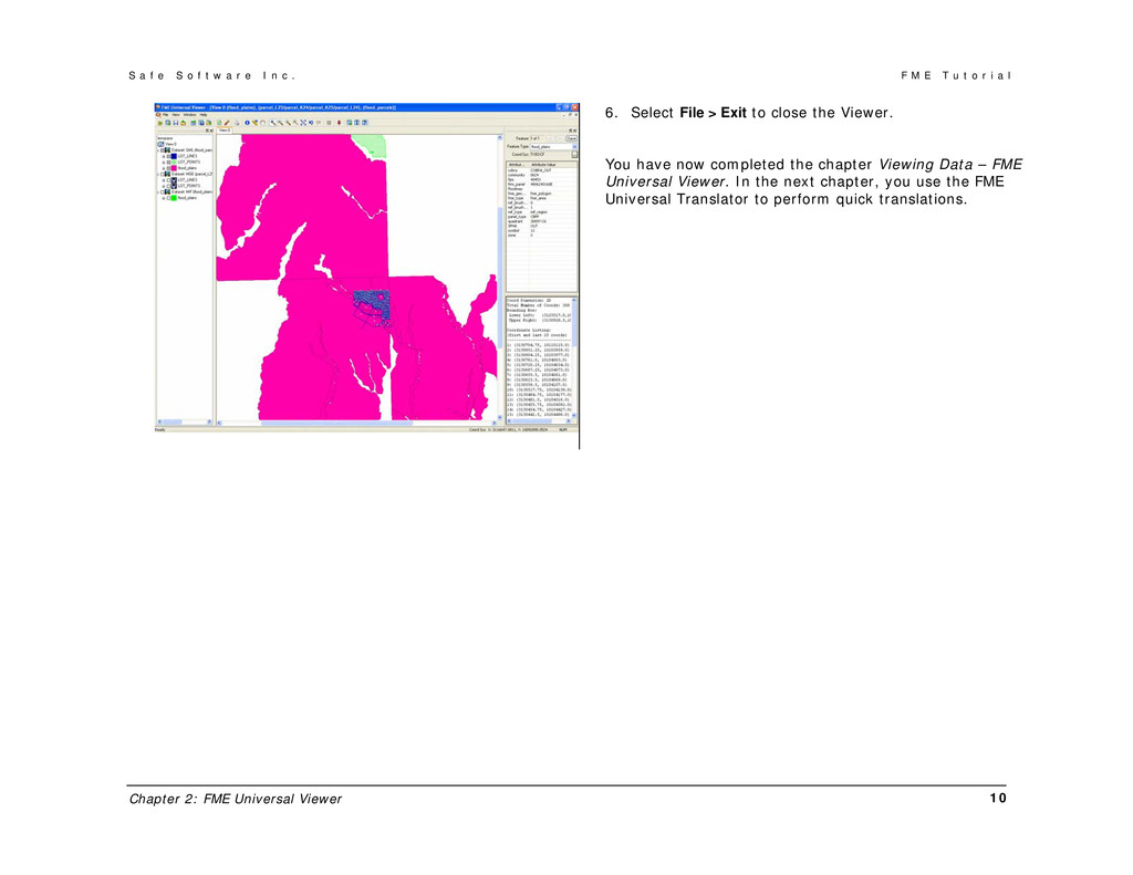
r e I n c . F M E T u t o r i a l Chapter 2: FME Universal Viewer 10 6. Select File > Exit to close the Viewer. You have now completed the chapter Viewing Data – FME Universal Viewer. In the next chapter, you use the FME Universal Translator to perform quick translations.
r e I n c . F M E T u t o r i a l Chapter 3: FME Universal Translator 11 Chapter 3 Quick Translations – FME Universal Translator In this chapter Automating translations Processing basic features Reprojecting data Objective In the previous exercise, you used the FME Universal Viewer to visualize data. You also learned how the Viewer is used for simple translations of small sections of the data. In this chapter, you use the Universal Translator in situations where it is not necessary to view the data; for example, when you only want to translate from one format to another, possibly transforming or reprojecting the data in the process. The FME Universal Translator is very useful in situations where the schema and geometry of the data do not have to change during the translation. Although you can the Universal Translator to make minor adjustments to datasets, the recommended tool for data manipulation is FME Workbench, which you can explore in Chapter 4.
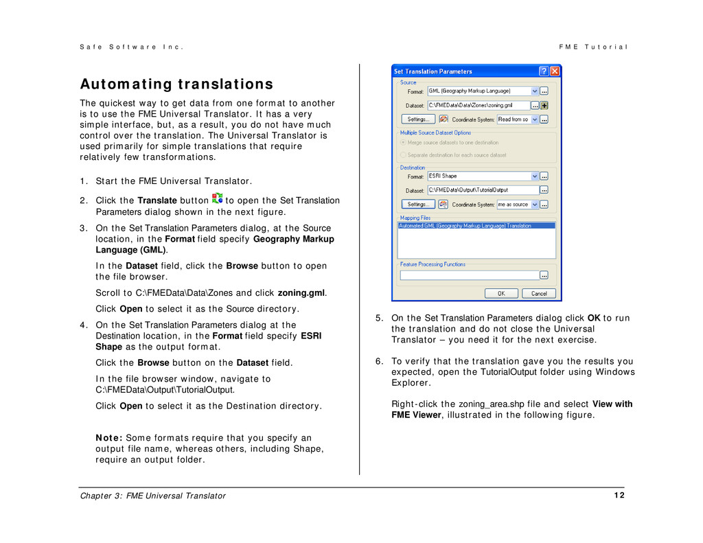
r e I n c . F M E T u t o r i a l Chapter 3: FME Universal Translator 12 Automating translations The quickest way to get data from one format to another is to use the FME Universal Translator. It has a very simple interface, but, as a result, you do not have much control over the translation. The Universal Translator is used primarily for simple translations that require relatively few transformations. 1. Start the FME Universal Translator. 2. Click the Translate button to open the Set Translation Parameters dialog shown in the next figure. 3. On the Set Translation Parameters dialog, at the Source location, in the Format field specify Geography Markup Language (GML). In the Dataset field, click the Browse button to open the file browser. Scroll to C:\FMEData\Data\Zones and click zoning.gml. Click Open to select it as the Source directory. 4. On the Set Translation Parameters dialog at the Destination location, in the Format field specify ESRI Shape as the output format. Click the Browse button on the Dataset field. In the file browser window, navigate to C:\FMEData\Output\TutorialOutput. Click Open to select it as the Destination directory. Note: Some formats require that you specify an output file name, whereas others, including Shape, require an output folder. 5. On the Set Translation Parameters dialog click OK to run the translation and do not close the Universal Translator – you need it for the next exercise. 6. To verify that the translation gave you the results you expected, open the TutorialOutput folder using Windows Explorer. Right-click the zoning_area.shp file and select View with FME Viewer, illustrated in the following figure.
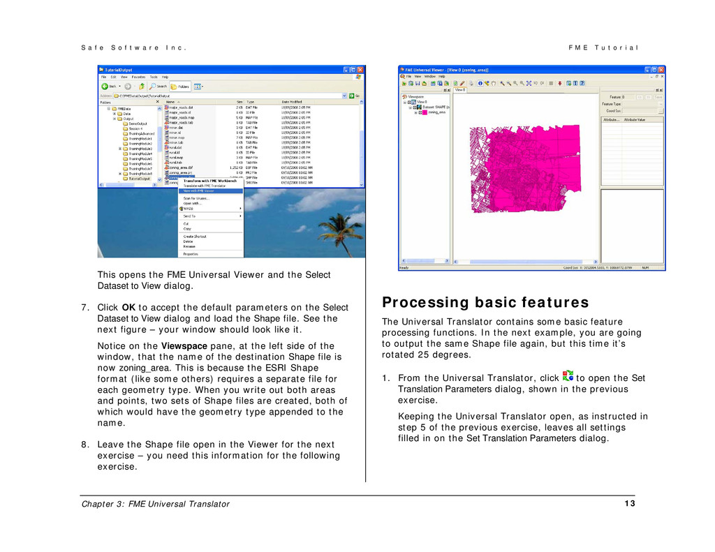
r e I n c . F M E T u t o r i a l Chapter 3: FME Universal Translator 13 This opens the FME Universal Viewer and the Select Dataset to View dialog. 7. Click OK to accept the default parameters on the Select Dataset to View dialog and load the Shape file. See the next figure – your window should look like it. Notice on the Viewspace pane, at the left side of the window, that the name of the destination Shape file is now zoning_area. This is because the ESRI Shape format (like some others) requires a separate file for each geometry type. When you write out both areas and points, two sets of Shape files are created, both of which would have the geometry type appended to the name. 8. Leave the Shape file open in the Viewer for the next exercise – you need this information for the following exercise. Processing basic features The Universal Translator contains some basic feature processing functions. In the next example, you are going to output the same Shape file again, but this time it’s rotated 25 degrees. 1. From the Universal Translator, click to open the Set Translation Parameters dialog, shown in the previous exercise. Keeping the Universal Translator open, as instructed in step 5 of the previous exercise, leaves all settings filled in on the Set Translation Parameters dialog.
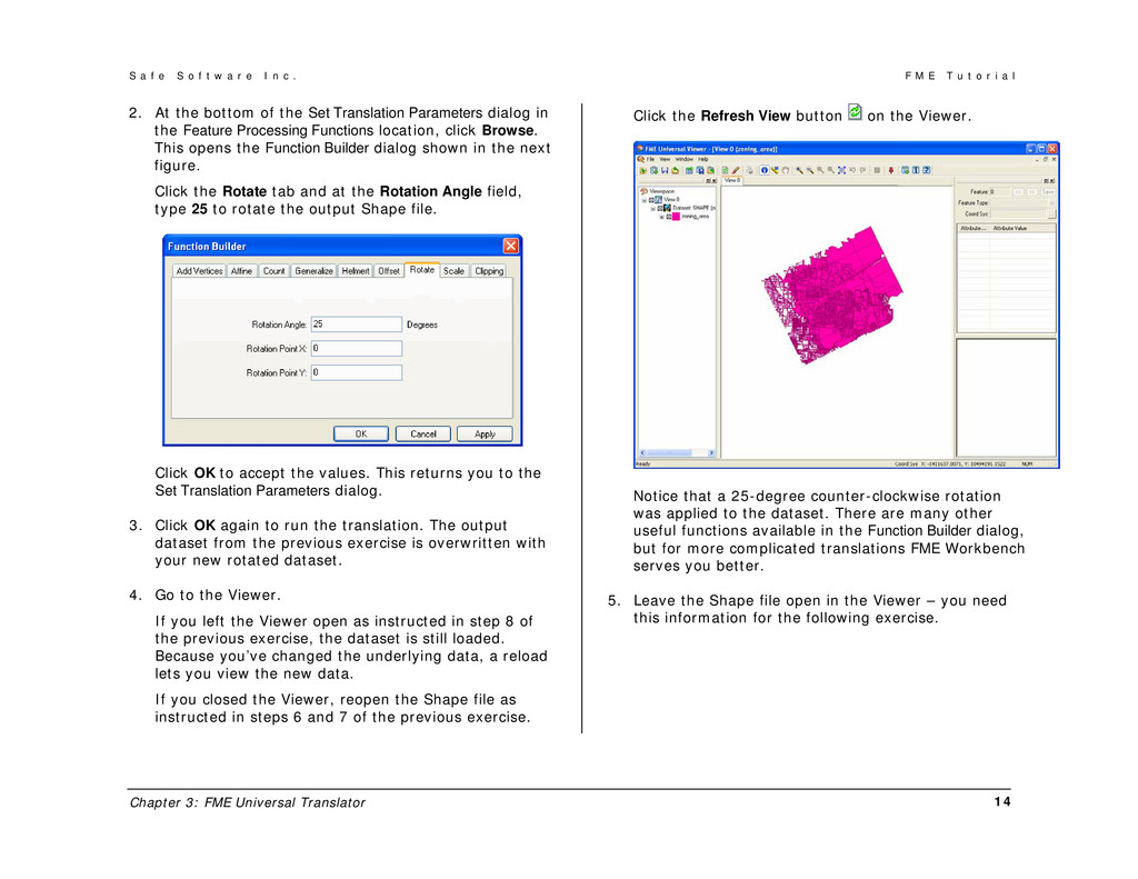
r e I n c . F M E T u t o r i a l Chapter 3: FME Universal Translator 14 2. At the bottom of the Set Translation Parameters dialog in the Feature Processing Functions location, click Browse. This opens the Function Builder dialog shown in the next figure. Click the Rotate tab and at the Rotation Angle field, type 25 to rotate the output Shape file. Click OK to accept the values. This returns you to the Set Translation Parameters dialog. 3. Click OK again to run the translation. The output dataset from the previous exercise is overwritten with your new rotated dataset. 4. Go to the Viewer. If you left the Viewer open as instructed in step 8 of the previous exercise, the dataset is still loaded. Because you’ve changed the underlying data, a reload lets you view the new data. If you closed the Viewer, reopen the Shape file as instructed in steps 6 and 7 of the previous exercise. Click the Refresh View button on the Viewer. Notice that a 25-degree counter-clockwise rotation was applied to the dataset. There are many other useful functions available in the Function Builder dialog, but for more complicated translations FME Workbench serves you better. 5. Leave the Shape file open in the Viewer – you need this information for the following exercise.
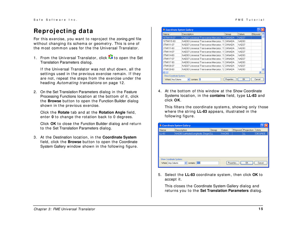
r e I n c . F M E T u t o r i a l Chapter 3: FME Universal Translator 15 Reprojecting data For this exercise, you want to reproject the zoning.gml file without changing its schema or geometry. This is one of the most common uses for the the Universal Translator. 1. From the Universal Translator, click to open the Set Translation Parameters dialog. If the Universal Translator was not shut down, all the settings used in the previous exercise remain. If they are not, repeat the steps from the exercise under the heading Automating translations on page 12. 2. On the Set Translation Parameters dialog in the Feature Processing Functions location at the bottom of it, click the Browse button to open the Function Builder dialog shown in the previous exercise. Click the Rotate tab and at the Rotation Angle field, enter 0 to change the rotation back to 0 degrees. Click OK to close the Function Builder dialog and return to the Set Translation Parameters dialog. 3. At the Destination location, in the Coordinate System field, click the Browse button to open the Coordinate System Gallery window shown in the following figure. 4. At the bottom of this window at the Show Coordinate Systems location, in the contains field, type LL-83 and click OK. This filters the coordinate systems, showing only those where the string LL-83 appears, illustrated in the following figure. 5. Select the LL-83 coordinate system, then click OK to accept it. This closes the Coordinate System Gallery dialog and returns you to the Set Translation Parameters dialog.
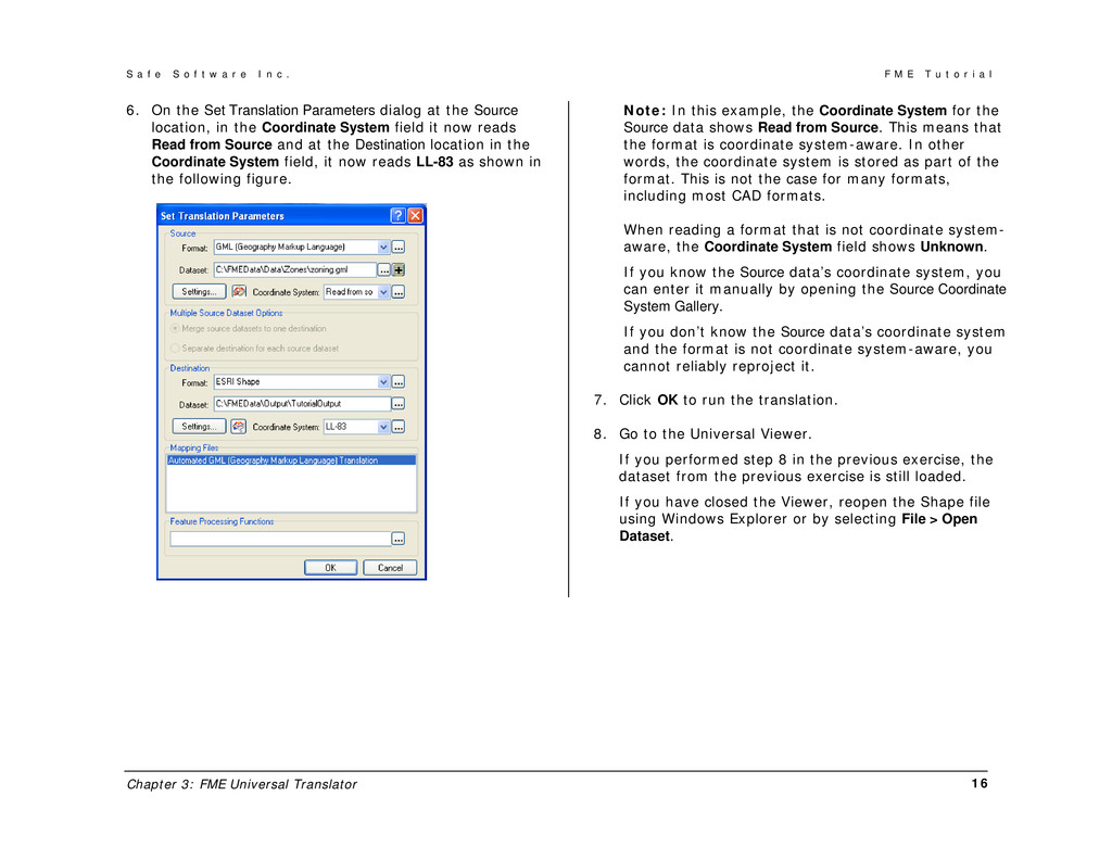
r e I n c . F M E T u t o r i a l Chapter 3: FME Universal Translator 16 6. On the Set Translation Parameters dialog at the Source location, in the Coordinate System field it now reads Read from Source and at the Destination location in the Coordinate System field, it now reads LL-83 as shown in the following figure. Note: In this example, the Coordinate System for the Source data shows Read from Source. This means that the format is coordinate system-aware. In other words, the coordinate system is stored as part of the format. This is not the case for many formats, including most CAD formats. When reading a format that is not coordinate system- aware, the Coordinate System field shows Unknown. If you know the Source data’s coordinate system, you can enter it manually by opening the Source Coordinate System Gallery. If you don’t know the Source data’s coordinate system and the format is not coordinate system-aware, you cannot reliably reproject it. 7. Click OK to run the translation. 8. Go to the Universal Viewer. If you performed step 8 in the previous exercise, the dataset from the previous exercise is still loaded. If you have closed the Viewer, reopen the Shape file using Windows Explorer or by selecting File > Open Dataset.
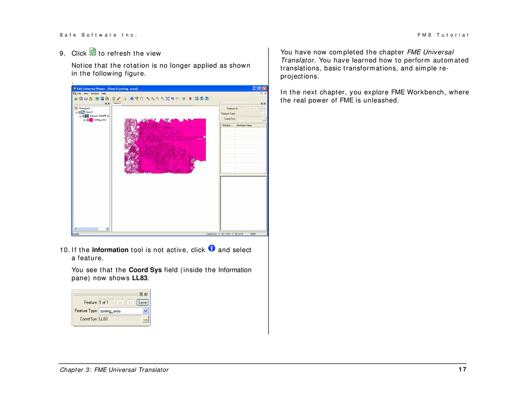
r e I n c . F M E T u t o r i a l Chapter 3: FME Universal Translator 17 9. Click to refresh the view Notice that the rotation is no longer applied as shown in the following figure. . 10. If the Information tool is not active, click and select a feature. You see that the Coord Sys field (inside the Information pane) now shows LL83. You have now completed the chapter FME Universal Translator. You have learned how to perform automated translations, basic transformations, and simple re- projections. In the next chapter, you explore FME Workbench, where the real power of FME is unleashed.
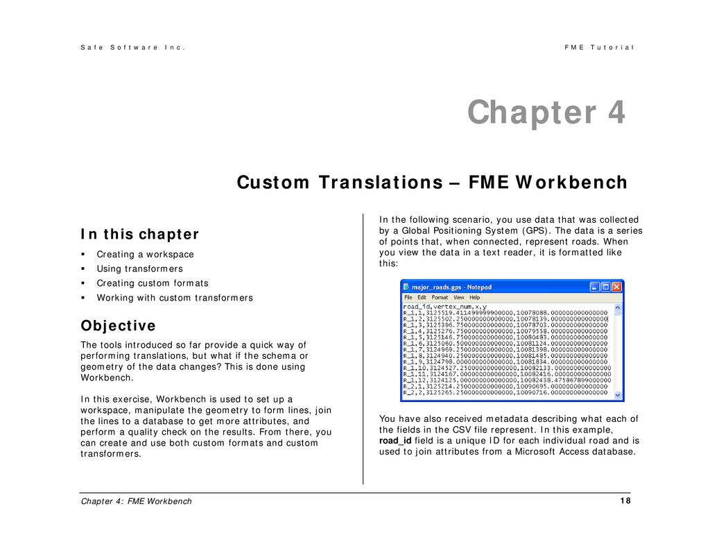
r e I n c . F M E T u t o r i a l Chapter 4: FME Workbench 18 Chapter 4 Custom Translations – FME Workbench In this chapter Creating a workspace Using transformers Creating custom formats Working with custom transformers Objective The tools introduced so far provide a quick way of performing translations, but what if the schema or geometry of the data changes? This is done using Workbench. In this exercise, Workbench is used to set up a workspace, manipulate the geometry to form lines, join the lines to a database to get more attributes, and perform a quality check on the results. From there, you can create and use both custom formats and custom transformers. In the following scenario, you use data that was collected by a Global Positioning System (GPS). The data is a series of points that, when connected, represent roads. When you view the data in a text reader, it is formatted like this: You have also received metadata describing what each of the fields in the CSV file represent. In this example, road_id field is a unique ID for each individual road and is used to join attributes from a Microsoft Access database.
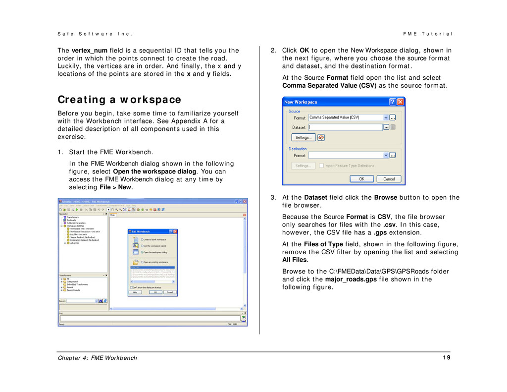
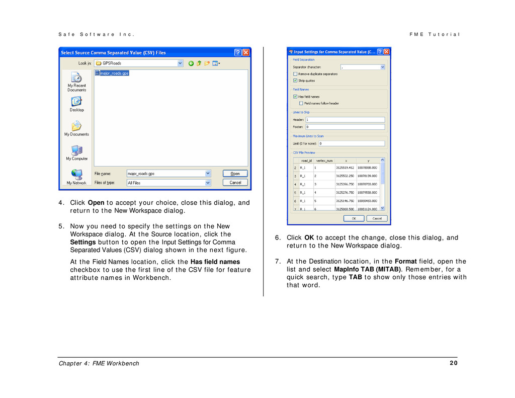
r e I n c . F M E T u t o r i a l Chapter 4: FME Workbench 19 The vertex_num field is a sequential ID that tells you the order in which the points connect to create the road. Luckily, the vertices are in order. And finally, the x and y locations of the points are stored in the x and y fields. Creating a workspace Before you begin, take some time to familiarize yourself with the Workbench interface. See Appendix A for a detailed description of all components used in this exercise. 1. Start the FME Workbench. In the FME Workbench dialog shown in the following figure, select Open the workspace dialog. You can access the FME Workbench dialog at any time by selecting File > New. 2. Click OK to open the New Workspace dialog, shown in the next figure, where you choose the source format and dataset, and the destination format. At the Source Format field open the list and select Comma Separated Value (CSV) as the source format. 3. At the Dataset field click the Browse button to open the file browser. Because the Source Format is CSV, the file browser only searches for files with the .csv. In this case, however, the CSV file has a .gps extension. At the Files of Type field, shown in the following figure, remove the CSV filter by opening the list and selecting All Files. Browse to the C:\FMEData\Data\GPS\GPSRoads folder and click the major_roads.gps file shown in the following figure.
r e I n c . F M E T u t o r i a l Chapter 4: FME Workbench 20 4. Click Open to accept your choice, close this dialog, and return to the New Workspace dialog. 5. Now you need to specify the settings on the New Workspace dialog. At the Source location, click the Settings button to open the Input Settings for Comma Separated Values (CSV) dialog shown in the next figure. At the Field Names location, click the Has field names checkbox to use the first line of the CSV file for feature attribute names in Workbench. 6. Click OK to accept the change, close this dialog, and return to the New Workspace dialog. 7. At the Destination location, in the Format field, open the list and select MapInfo TAB (MITAB). Remember, for a quick search, type TAB to show only those entries with that word.
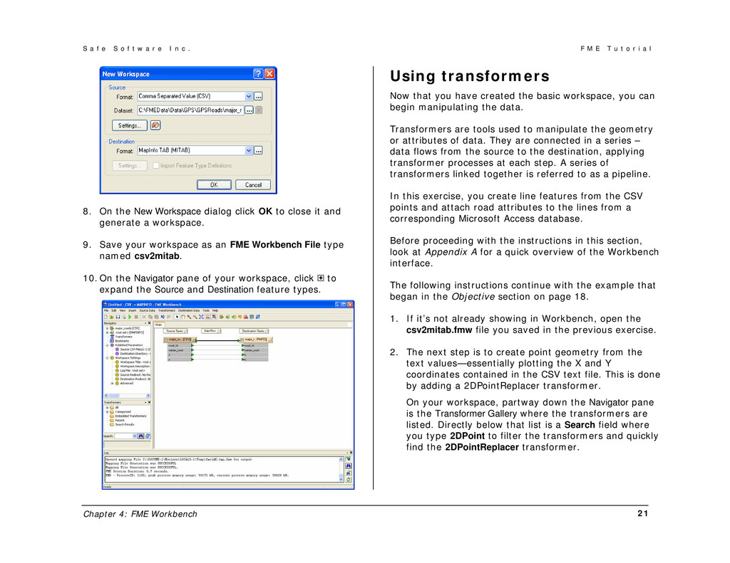
r e I n c . F M E T u t o r i a l Chapter 4: FME Workbench 21 8. On the New Workspace dialog click OK to close it and generate a workspace. 9. Save your workspace as an FME Workbench File type named csv2mitab. 10. On the Navigator pane of your workspace, click to expand the Source and Destination feature types. Using transformers Now that you have created the basic workspace, you can begin manipulating the data. Transformers are tools used to manipulate the geometry or attributes of data. They are connected in a series – data flows from the source to the destination, applying transformer processes at each step. A series of transformers linked together is referred to as a pipeline. In this exercise, you create line features from the CSV points and attach road attributes to the lines from a corresponding Microsoft Access database. Before proceeding with the instructions in this section, look at Appendix A for a quick overview of the Workbench interface. The following instructions continue with the example that began in the Objective section on page 18. 1. If it’s not already showing in Workbench, open the csv2mitab.fmw file you saved in the previous exercise. 2. The next step is to create point geometry from the text values—essentially plotting the X and Y coordinates contained in the CSV text file. This is done by adding a 2DPointReplacer transformer. On your workspace, partway down the Navigator pane is the Transformer Gallery where the transformers are listed. Directly below that list is a Search field where you type 2DPoint to filter the transformers and quickly find the 2DPointReplacer transformer.
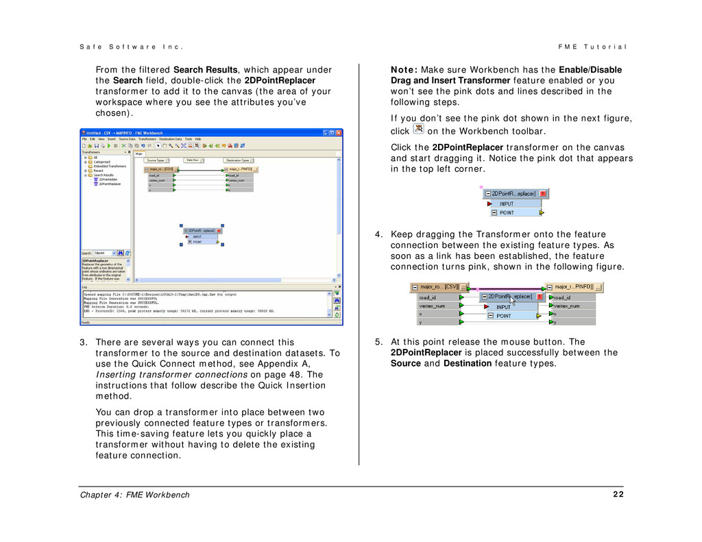
r e I n c . F M E T u t o r i a l Chapter 4: FME Workbench 22 From the filtered Search Results, which appear under the Search field, double-click the 2DPointReplacer transformer to add it to the canvas (the area of your workspace where you see the attributes you’ve chosen). 3. There are several ways you can connect this transformer to the source and destination datasets. To use the Quick Connect method, see Appendix A, Inserting transformer connections on page 48. The instructions that follow describe the Quick Insertion method. You can drop a transformer into place between two previously connected feature types or transformers. This time-saving feature lets you quickly place a transformer without having to delete the existing feature connection. Note: Make sure Workbench has the Enable/Disable Drag and Insert Transformer feature enabled or you won’t see the pink dots and lines described in the following steps. If you don’t see the pink dot shown in the next figure, click on the Workbench toolbar. Click the 2DPointReplacer transformer on the canvas and start dragging it. Notice the pink dot that appears in the top left corner. 4. Keep dragging the Transformer onto the feature connection between the existing feature types. As soon as a link has been established, the feature connection turns pink, shown in the following figure. 5. At this point release the mouse button. The 2DPointReplacer is placed successfully between the Source and Destination feature types.
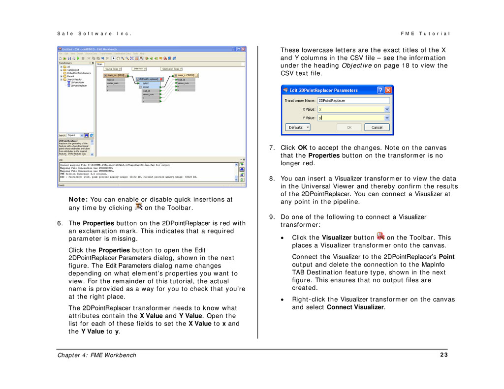
r e I n c . F M E T u t o r i a l Chapter 4: FME Workbench 23 Note: You can enable or disable quick insertions at any time by clicking on the Toolbar. 6. The Properties button on the 2DPointReplacer is red with an exclamation mark. This indicates that a required parameter is missing. Click the Properties button to open the Edit 2DPointReplacer Parameters dialog, shown in the next figure. The Edit Parameters dialog name changes depending on what element’s properties you want to view. For the remainder of this tutorial, the actual name is provided as a way for you to check that you’re at the right place. The 2DPointReplacer transformer needs to know what attributes contain the X Value and Y Value. Open the list for each of these fields to set the X Value to x and the Y Value to y. These lowercase letters are the exact titles of the X and Y columns in the CSV file – see the information under the heading Objective on page 18 to view the CSV text file. 7. Click OK to accept the changes. Note on the canvas that the Properties button on the transformer is no longer red. 8. You can insert a Visualizer transformer to view the data in the Universal Viewer and thereby confirm the results of the 2DPointReplacer. You can connect a Visualizer at any point in the pipeline. 9. Do one of the following to connect a Visualizer transformer: • Click the Visualizer button on the Toolbar. This places a Visualizer transformer onto the canvas. Connect the Visualizer to the 2DPointReplacer’s Point output and delete the connection to the MapInfo TAB Destination feature type, shown in the next figure. This ensures that no output files are created. • Right-click the Visualizer transformer on the canvas and select Connect Visualizer.
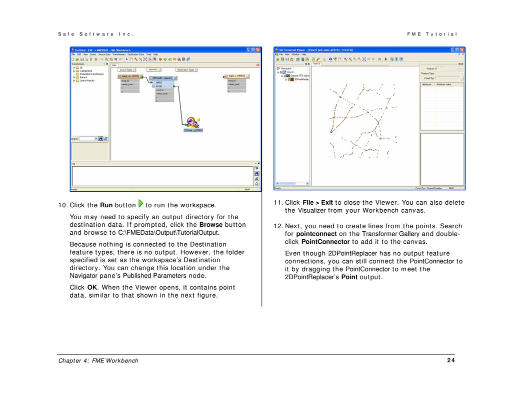
r e I n c . F M E T u t o r i a l Chapter 4: FME Workbench 24 10. Click the Run button to run the workspace. You may need to specify an output directory for the destination data. If prompted, click the Browse button and browse to C:\FMEData\Output\TutorialOutput. Because nothing is connected to the Destination feature types, there is no output. However, the folder specified is set as the workspace’s Destination directory. You can change this location under the Navigator pane’s Published Parameters node. Click OK. When the Viewer opens, it contains point data, similar to that shown in the next figure. 11. Click File > Exit to close the Viewer. You can also delete the Visualizer from your Workbench canvas. 12. Next, you need to create lines from the points. Search for pointconnect on the Transformer Gallery and double- click PointConnector to add it to the canvas. Even though 2DPointReplacer has no output feature connections, you can still connect the PointConnector to it by dragging the PointConnector to meet the 2DPointReplacer’s Point output.
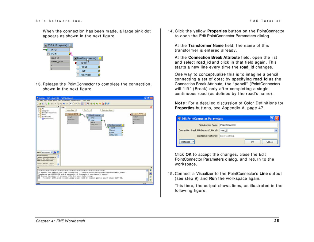
r e I n c . F M E T u t o r i a l Chapter 4: FME Workbench 25 When the connection has been made, a large pink dot appears as shown in the next figure. 13. Release the PointConnector to complete the connection, shown in the next figure. 14. Click the yellow Properties button on the PointConnector to open the Edit PointConnector Parameters dialog. At the Transformer Name field, the name of this transformer is entered already. At the Connection Break Attribute field, open the list and select road_id and click in that field again. This starts a new line every time the road_id changes. One way to conceptualize this is to imagine a pencil connecting a set of dots; by specifying road_id as the Connection Break Attribute, the “pencil” (PointConnector) will “lift” (Break) only after completing a single continuous road (as defined by the road’s name). Note: For a detailed discussion of Color Definitions for Properties buttons, see Appendix A, page 47. Click OK to accept the changes, close the Edit PointConnector Parameters dialog, and return to the workspace. 15. Connect a Visualizer to the PointConnector’s Line output (see step 9) and Run the workspace again. This time, the output shows lines, as illustrated in the following figure.
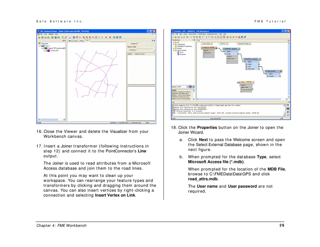
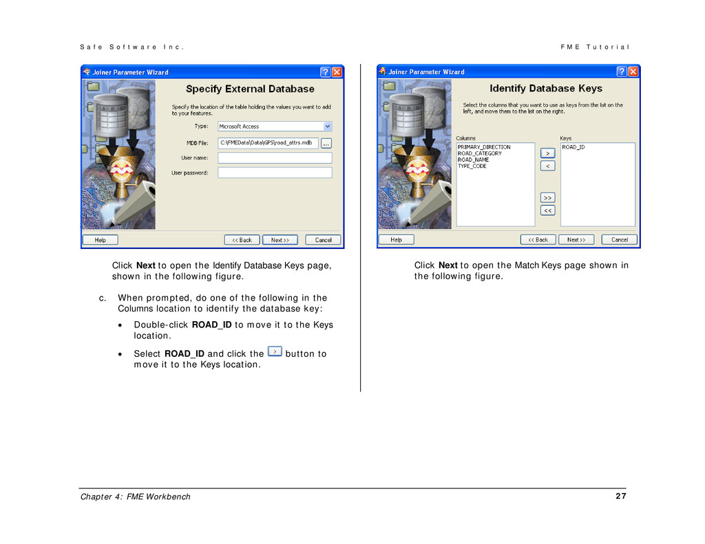
r e I n c . F M E T u t o r i a l Chapter 4: FME Workbench 26 16. Close the Viewer and delete the Visualizer from your Workbench canvas. 17. Insert a Joiner transformer (following instructions in step 12) and connect it to the PointConnector’s Line output. The Joiner is used to read attributes from a Microsoft Access database and join them to the road lines. At this point you may want to clean up your workspace. You can rearrange your feature types and transformers by clicking and dragging them around the canvas. You can also insert vertices by right-clicking a connection and selecting Insert Vertex on Link. 18. Click the Properties button on the Joiner to open the Joiner Wizard. a. Click Next to pass the Welcome screen and open the Select External Database page, shown in the next figure. b. When prompted for the database Type, select Microsoft Access file (*.mdb). When prompted for the location of the MDB File, browse to C:\FMEData\Data\GPS and click road_attrs.mdb. The User name and User password are not required.
r e I n c . F M E T u t o r i a l Chapter 4: FME Workbench 27 Click Next to open the Identify Database Keys page, shown in the following figure. c. When prompted, do one of the following in the Columns location to identify the database key: • Double-click ROAD_ID to move it to the Keys location. • Select ROAD_ID and click the button to move it to the Keys location. Click Next to open the Match Keys page shown in the following figure.
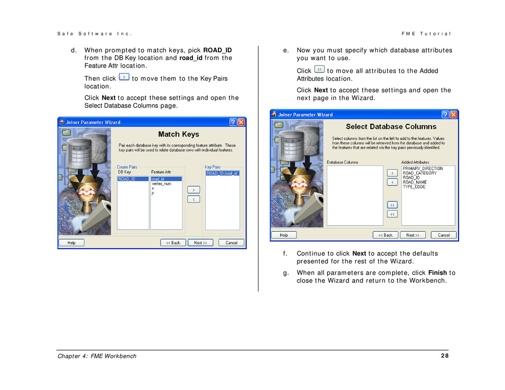
r e I n c . F M E T u t o r i a l Chapter 4: FME Workbench 28 d. When prompted to match keys, pick ROAD_ID from the DB Key location and road_id from the Feature Attr location. Then click to move them to the Key Pairs location. Click Next to accept these settings and open the Select Database Columns page. e. Now you must specify which database attributes you want to use. Click to move all attributes to the Added Attributes location. Click Next to accept these settings and open the next page in the Wizard. f. Continue to click Next to accept the defaults presented for the rest of the Wizard. g. When all parameters are complete, click Finish to close the Wizard and return to the Workbench.
r e I n c . F M E T u t o r i a l Chapter 4: FME Workbench 29 19. Expand the Joined output of the Joiner by clicking to its left. This shows the newly added attribute names. 20. This is a good time to save your workspace. Do so by selecting File > Save As. Name the workspace CSVRoads.fmw and save it under My Documents\My FME Workspaces. 21. Insert an AttributeFilter and connect the Joined output from the Joiner to it, shown in the next figure. The AttributeFilter transformer lets you classify your roads based on an attribute value. You may want to rearrange your workspace again before proceeding. 22. Click the Properties button on the AttributeFilter. On the Edit AttributeFilter Parameters dialog (shown in the following figure) at the Attribute to filter by field, open the list and select ROAD_CATEGORY. At the Possible Attribute Values location, type RURAL on the first line, MAJOR on the second line, and MINOR on the third line. Tip: If you are unsure of all the possible attribute values for ROAD_CATEGORY use the Import button at the lower right of your workspace. It prompts you to provide a source dataset to read the attribute schema from (in this case, Microsoft Access Database) and to browse to the file that contains the data (in this case, road_attrs.mdb). Workbench then reads the file, searches for all unique values for that particular
r e I n c . F M E T u t o r i a l Chapter 4: FME Workbench 30 attribute, and populates the Possible Attribute Values table automatically. 23. On the Edit AttributeFilter Parameters dialog click OK. Notice on your canvas that the AttributeFilter has RURAL, MAJOR, and MINOR outputs. Connect a Visualizer to the AttributeFilter MAJOR output and Run the workspace. See the following figure for a look at the results. The Viewer shows you only those features where road_category = MAJOR. Close the Viewer and delete the Visualizer in Workbench. 24. On your workspace under Destination types, if it’s not already opened, expand the Destination feature type by clicking . Notice that it does not contain any attribute definitions from the database you have just joined to. There are several options to correct this, however, in this case the best way is to import a new Destination feature type using roads_attrs.mdb as the template for the attribute schema.
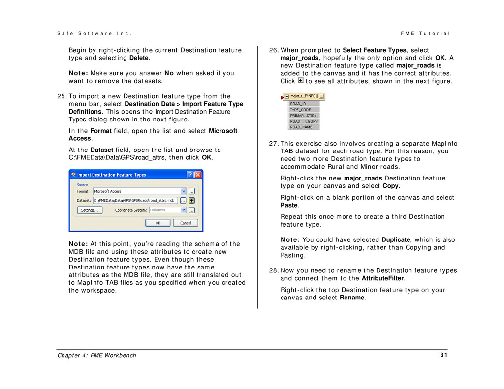
r e I n c . F M E T u t o r i a l Chapter 4: FME Workbench 31 Begin by right-clicking the current Destination feature type and selecting Delete. Note: Make sure you answer No when asked if you want to remove the datasets. 25. To import a new Destination feature type from the menu bar, select Destination Data > Import Feature Type Definitions. This opens the Import Destination Feature Types dialog shown in the next figure. In the Format field, open the list and select Microsoft Access. At the Dataset field, open the list and browse to C:\FMEData\Data\GPS\road_attrs, then click OK. Note: At this point, you’re reading the schema of the MDB file and using these attributes to create new Destination feature types. Even though these Destination feature types now have the same attributes as the MDB file, they are still translated out to MapInfo TAB files as you specified when you created the workspace. 26. When prompted to Select Feature Types, select major_roads, hopefully the only option and click OK. A new Destination feature type called major_roads is added to the canvas and it has the correct attributes. Click to see all attributes, shown in the next figure. 27. This exercise also involves creating a separate MapInfo TAB dataset for each road type. For this reason, you need two more Destination feature types to accommodate Rural and Minor roads. Right-click the new major_roads Destination feature type on your canvas and select Copy. Right-click on a blank portion of the canvas and select Paste. Repeat this once more to create a third Destination feature type. Note: You could have selected Duplicate, which is also available by right-clicking, rather than Copying and Pasting. 28. Now you need to rename the Destination feature types and connect them to the AttributeFilter. Right-click the top Destination feature type on your canvas and select Rename.
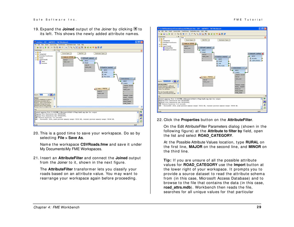
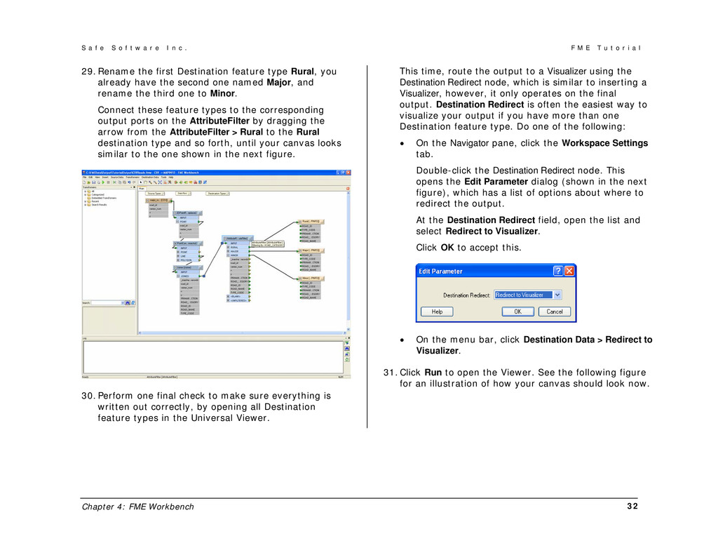
r e I n c . F M E T u t o r i a l Chapter 4: FME Workbench 32 29. Rename the first Destination feature type Rural, you already have the second one named Major, and rename the third one to Minor. Connect these feature types to the corresponding output ports on the AttributeFilter by dragging the arrow from the AttributeFilter > Rural to the Rural destination type and so forth, until your canvas looks similar to the one shown in the next figure. 30. Perform one final check to make sure everything is written out correctly, by opening all Destination feature types in the Universal Viewer. This time, route the output to a Visualizer using the Destination Redirect node, which is similar to inserting a Visualizer, however, it only operates on the final output. Destination Redirect is often the easiest way to visualize your output if you have more than one Destination feature type. Do one of the following: • On the Navigator pane, click the Workspace Settings tab. Double-click the Destination Redirect node. This opens the Edit Parameter dialog (shown in the next figure), which has a list of options about where to redirect the output. At the Destination Redirect field, open the list and select Redirect to Visualizer. Click OK to accept this. • On the menu bar, click Destination Data > Redirect to Visualizer. 31. Click Run to open the Viewer. See the following figure for an illustration of how your canvas should look now.
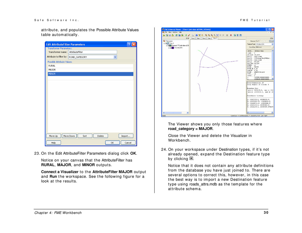
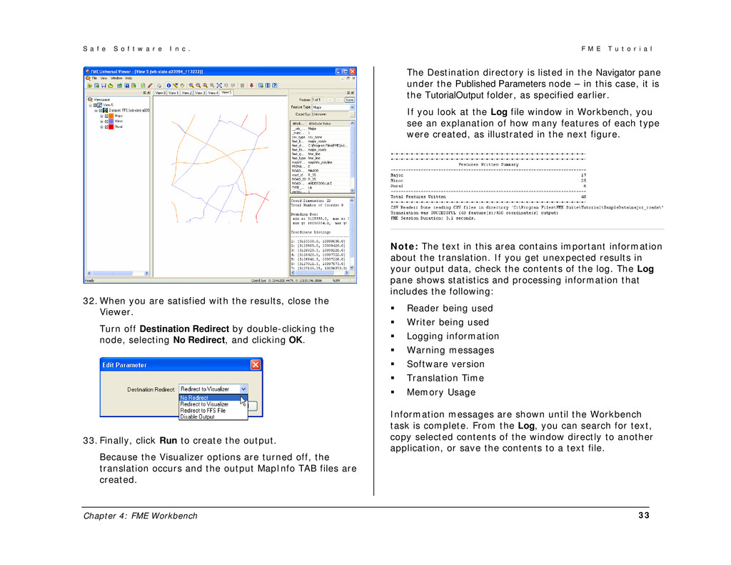
r e I n c . F M E T u t o r i a l Chapter 4: FME Workbench 33 32. When you are satisfied with the results, close the Viewer. Turn off Destination Redirect by double-clicking the node, selecting No Redirect, and clicking OK. 33. Finally, click Run to create the output. Because the Visualizer options are turned off, the translation occurs and the output MapInfo TAB files are created. The Destination directory is listed in the Navigator pane under the Published Parameters node – in this case, it is the TutorialOutput folder, as specified earlier. If you look at the Log file window in Workbench, you see an explanation of how many features of each type were created, as illustrated in the next figure. Note: The text in this area contains important information about the translation. If you get unexpected results in your output data, check the contents of the log. The Log pane shows statistics and processing information that includes the following: Reader being used Writer being used Logging information Warning messages Software version Translation Time Memory Usage Information messages are shown until the Workbench task is complete. From the Log, you can search for text, copy selected contents of the window directly to another application, or save the contents to a text file.
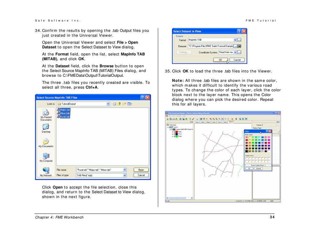
r e I n c . F M E T u t o r i a l Chapter 4: FME Workbench 34 34. Confirm the results by opening the .tab Output files you just created in the Universal Viewer. Open the Universal Viewer and select File > Open Dataset to open the Select Dataset to View dialog. At the Format field, open the list, select MapInfo TAB (MITAB), and click OK. At the Dataset field, click the Browse button to open the Select Source MapInfo TAB (MITAB) Files dialog, and browse to C:\FMEData\Output\TutorialOutput. The three .tab files you recently created are visible. To select all three, press Ctrl+A. Click Open to accept the file selection, close this dialog, and return to the Select Dataset to View dialog, shown in the next figure. 35. Click OK to load the three .tab files into the Viewer. Note: All three .tab files are shown in the same color, which makes it difficult to identify the various road types. To change the color of each layer, click the color block next to the layer name. This opens the Color dialog where you can pick the desired color. Repeat this for all layers.
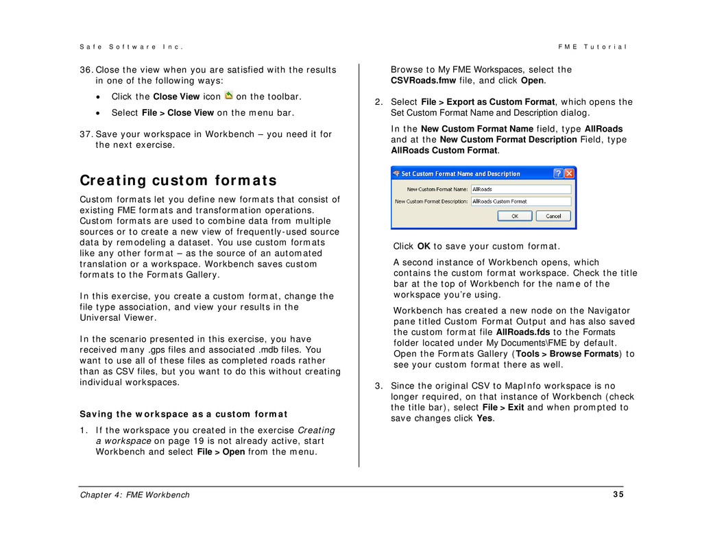
r e I n c . F M E T u t o r i a l Chapter 4: FME Workbench 35 36. Close the view when you are satisfied with the results in one of the following ways: • Click the Close View icon on the toolbar. • Select File > Close View on the menu bar. 37. Save your workspace in Workbench – you need it for the next exercise. Creating custom formats Custom formats let you define new formats that consist of existing FME formats and transformation operations. Custom formats are used to combine data from multiple sources or to create a new view of frequently-used source data by remodeling a dataset. You use custom formats like any other format – as the source of an automated translation or a workspace. Workbench saves custom formats to the Formats Gallery. In this exercise, you create a custom format, change the file type association, and view your results in the Universal Viewer. In the scenario presented in this exercise, you have received many .gps files and associated .mdb files. You want to use all of these files as completed roads rather than as CSV files, but you want to do this without creating individual workspaces. Saving the workspace as a custom format 1. If the workspace you created in the exercise Creating a workspace on page 19 is not already active, start Workbench and select File > Open from the menu. Browse to My FME Workspaces, select the CSVRoads.fmw file, and click Open. 2. Select File > Export as Custom Format, which opens the Set Custom Format Name and Description dialog. In the New Custom Format Name field, type AllRoads and at the New Custom Format Description Field, type AllRoads Custom Format. Click OK to save your custom format. A second instance of Workbench opens, which contains the custom format workspace. Check the title bar at the top of Workbench for the name of the workspace you’re using. Workbench has created a new node on the Navigator pane titled Custom Format Output and has also saved the custom format file AllRoads.fds to the Formats folder located under My Documents\FME by default. Open the Formats Gallery (Tools > Browse Formats) to see your custom format there as well. 3. Since the original CSV to MapInfo workspace is no longer required, on that instance of Workbench (check the title bar), select File > Exit and when prompted to save changes click Yes.
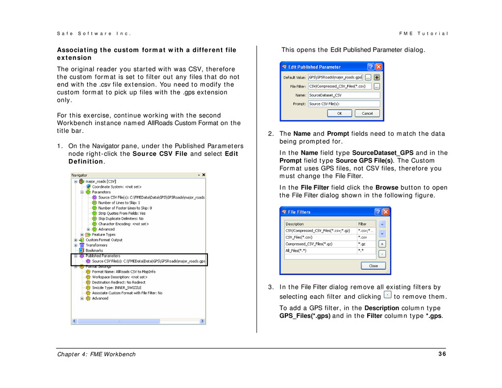
r e I n c . F M E T u t o r i a l Chapter 4: FME Workbench 36 Associating the custom format with a different file extension The original reader you started with was CSV, therefore the custom format is set to filter out any files that do not end with the .csv file extension. You need to modify the custom format to pick up files with the .gps extension only. For this exercise, continue working with the second Workbench instance named AllRoads Custom Format on the title bar. 1. On the Navigator pane, under the Published Parameters node right-click the Source CSV File and select Edit Definition. This opens the Edit Published Parameter dialog. 2. The Name and Prompt fields need to match the data being prompted for. In the Name field type SourceDataset_GPS and in the Prompt field type Source GPS File(s). The Custom Format uses GPS files, not CSV files, therefore you must change the File Filter. In the File Filter field click the Browse button to open the File Filter dialog shown in the following figure. 3. In the File Filter dialog remove all existing filters by selecting each filter and clicking to remove them. To add a GPS filter, in the Description column type GPS_Files(*.gps) and in the Filter column type *.gps.
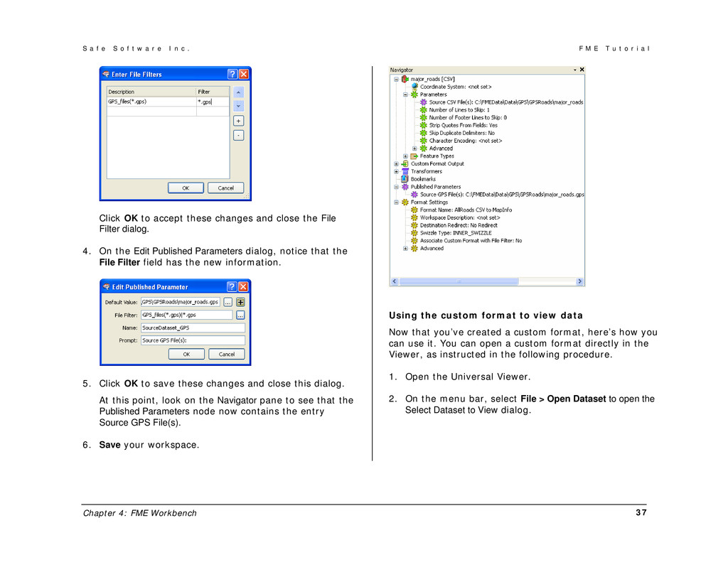
r e I n c . F M E T u t o r i a l Chapter 4: FME Workbench 37 Click OK to accept these changes and close the File Filter dialog. 4. On the Edit Published Parameters dialog, notice that the File Filter field has the new information. 5. Click OK to save these changes and close this dialog. At this point, look on the Navigator pane to see that the Published Parameters node now contains the entry Source GPS File(s). 6. Save your workspace. Using the custom format to view data Now that you’ve created a custom format, here’s how you can use it. You can open a custom format directly in the Viewer, as instructed in the following procedure. 1. Open the Universal Viewer. 2. On the menu bar, select File > Open Dataset to open the Select Dataset to View dialog.
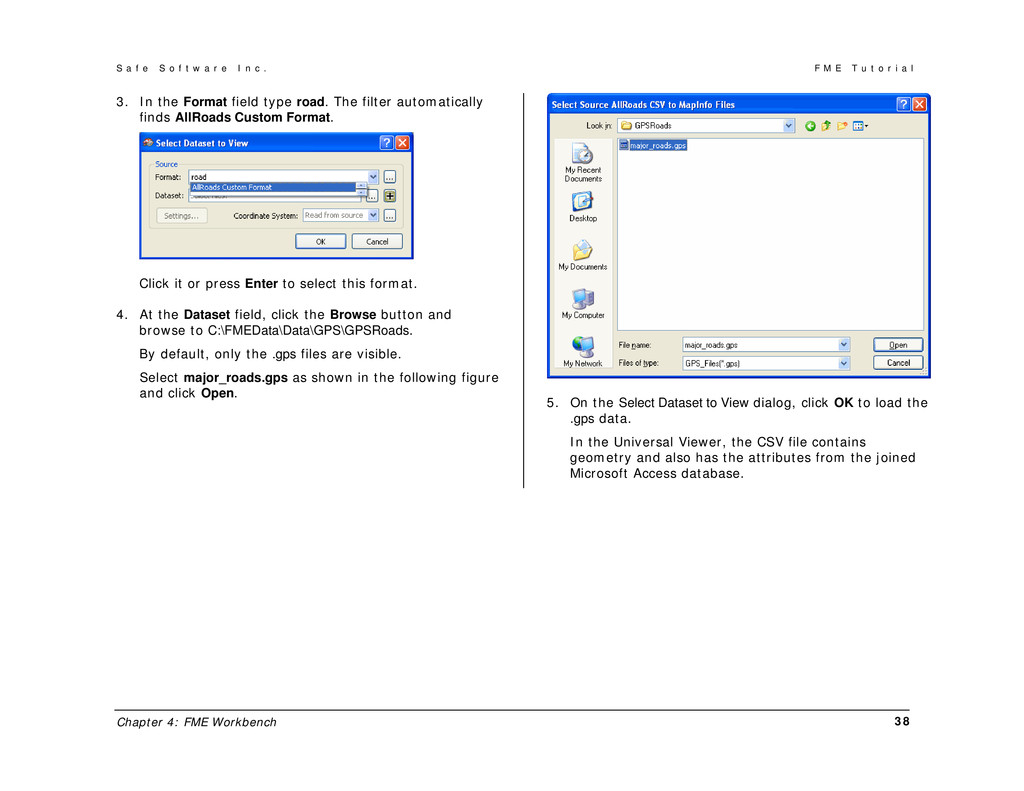
r e I n c . F M E T u t o r i a l Chapter 4: FME Workbench 38 3. In the Format field type road. The filter automatically finds AllRoads Custom Format. Click it or press Enter to select this format. 4. At the Dataset field, click the Browse button and browse to C:\FMEData\Data\GPS\GPSRoads. By default, only the .gps files are visible. Select major_roads.gps as shown in the following figure and click Open. 5. On the Select Dataset to View dialog, click OK to load the .gps data. In the Universal Viewer, the CSV file contains geometry and also has the attributes from the joined Microsoft Access database.
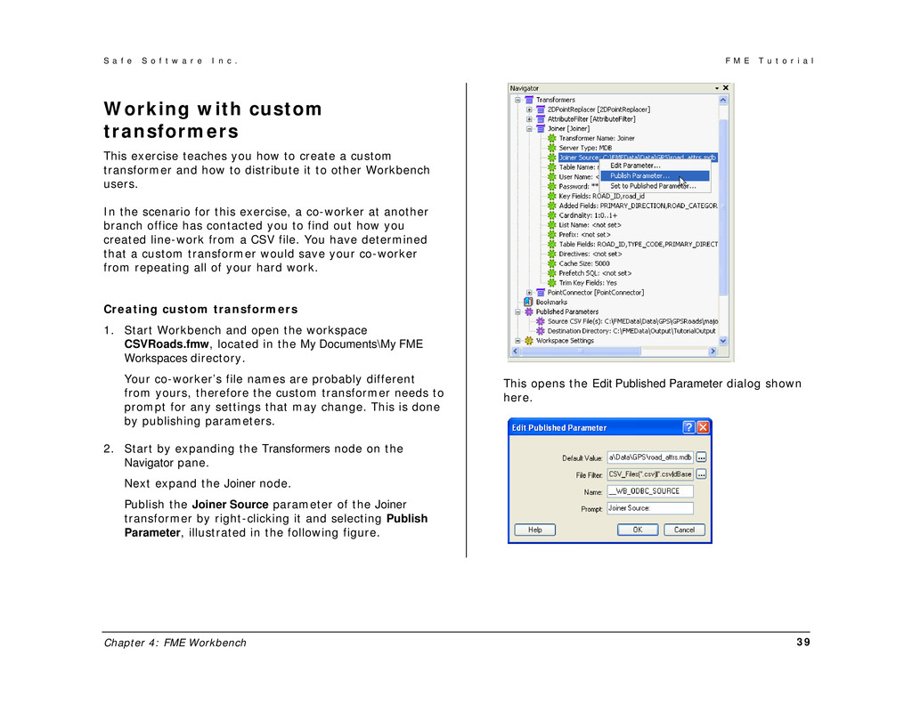
r e I n c . F M E T u t o r i a l Chapter 4: FME Workbench 39 Working with custom transformers This exercise teaches you how to create a custom transformer and how to distribute it to other Workbench users. In the scenario for this exercise, a co-worker at another branch office has contacted you to find out how you created line-work from a CSV file. You have determined that a custom transformer would save your co-worker from repeating all of your hard work. Creating custom transformers 1. Start Workbench and open the workspace CSVRoads.fmw, located in the My Documents\My FME Workspaces directory. Your co-worker’s file names are probably different from yours, therefore the custom transformer needs to prompt for any settings that may change. This is done by publishing parameters. 2. Start by expanding the Transformers node on the Navigator pane. Next expand the Joiner node. Publish the Joiner Source parameter of the Joiner transformer by right-clicking it and selecting Publish Parameter, illustrated in the following figure. This opens the Edit Published Parameter dialog shown here.
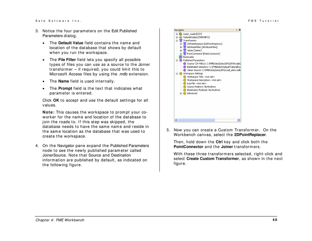
r e I n c . F M E T u t o r i a l Chapter 4: FME Workbench 40 3. Notice the four parameters on the Edit Published Parameters dialog. • The Default Value field contains the name and location of the database that shows by default when you run the workspace. • The File Filter field lets you specify all possible types of files you can use as a source to the Joiner transformer – if required, you could limit this to Microsoft Access files by using the .mdb extension. • The Name field is used internally. • The Prompt field is the text that indicates what parameter is entered. Click OK to accept and use the default settings for all values. Note: This causes the workspace to prompt your co- worker for the name and location of the database to join the roads to. If this step was skipped, the database needs to have the same name and reside in the same location as the database that was used to create the workspace. 4. On the Navigator pane expand the Published Parameters node to see the newly published parameter called JoinerSource. Note that Source and Destination information are published by default, as indicated on the following figure. 5. Now you can create a Custom Transformer. On the Workbench canvas, select the 2DPointReplacer. Then, hold down the Ctrl key and click both the PointConnector and the Joiner transformers. With these three transformers selected, right-click and select Create Custom Transformer, as shown in the next figure.
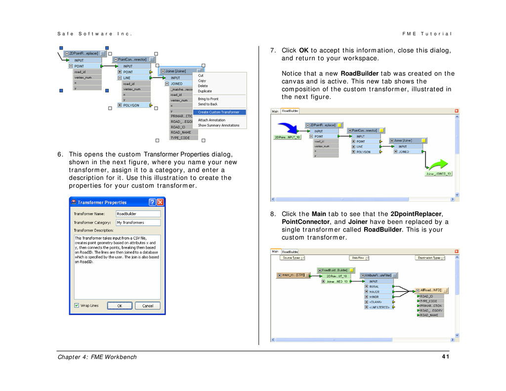
r e I n c . F M E T u t o r i a l Chapter 4: FME Workbench 41 6. This opens the custom Transformer Properties dialog, shown in the next figure, where you name your new transformer, assign it to a category, and enter a description for it. Use this illustration to create the properties for your custom transformer. 7. Click OK to accept this information, close this dialog, and return to your workspace. Notice that a new RoadBuilder tab was created on the canvas and is active. This new tab shows the composition of the custom transformer, illustrated in the next figure. 8. Click the Main tab to see that the 2DpointReplacer, PointConnector, and Joiner have been replaced by a single transformer called RoadBuilder. This is your custom transformer.
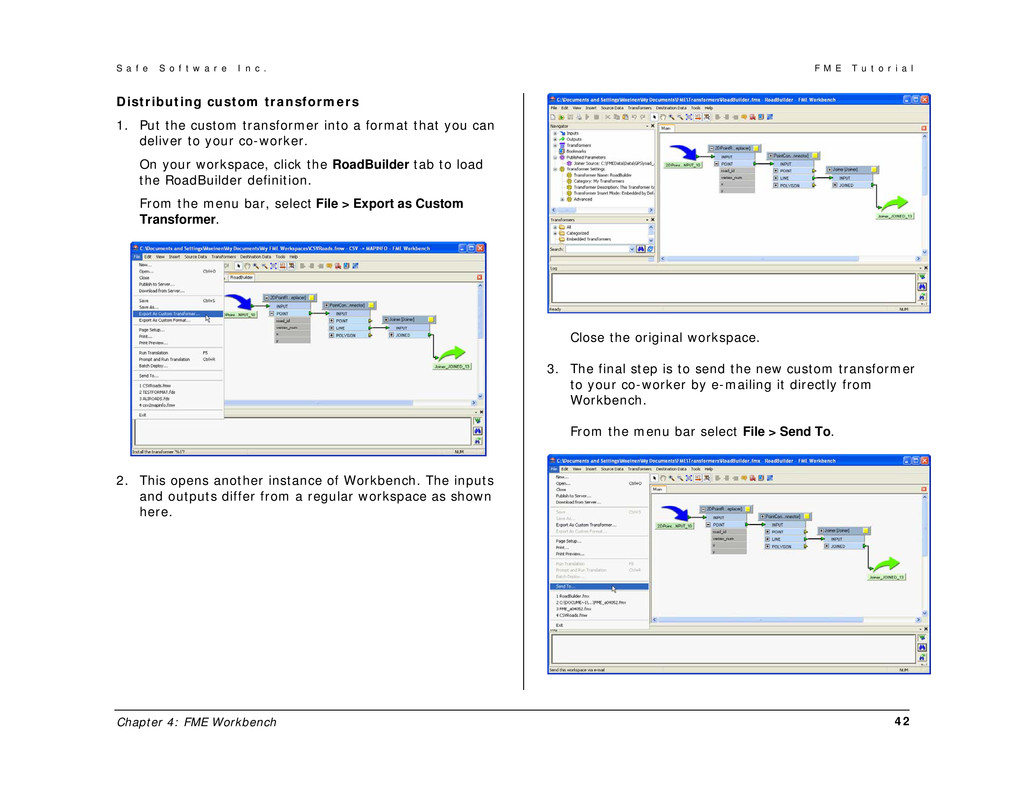
r e I n c . F M E T u t o r i a l Chapter 4: FME Workbench 42 Distributing custom transformers 1. Put the custom transformer into a format that you can deliver to your co-worker. On your workspace, click the RoadBuilder tab to load the RoadBuilder definition. From the menu bar, select File > Export as Custom Transformer. 2. This opens another instance of Workbench. The inputs and outputs differ from a regular workspace as shown here. Close the original workspace. 3. The final step is to send the new custom transformer to your co-worker by e-mailing it directly from Workbench. From the menu bar select File > Send To.
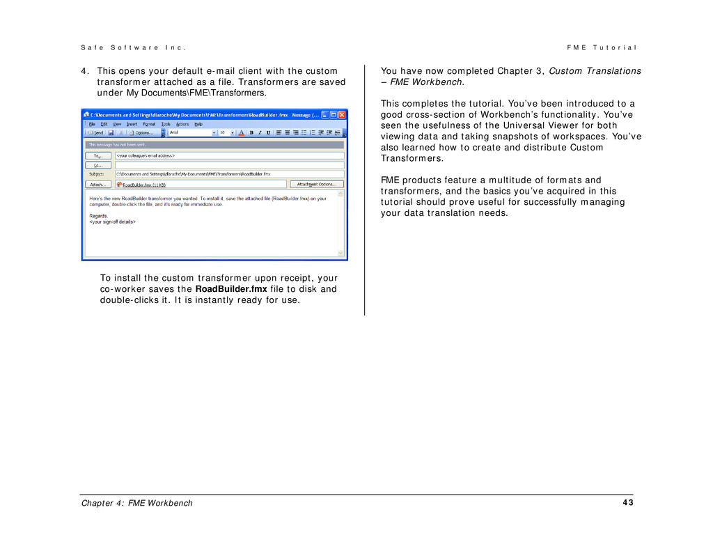
r e I n c . F M E T u t o r i a l Chapter 4: FME Workbench 43 4. This opens your default e-mail client with the custom transformer attached as a file. Transformers are saved under My Documents\FME\Transformers. To install the custom transformer upon receipt, your co-worker saves the RoadBuilder.fmx file to disk and double-clicks it. It is instantly ready for use. You have now completed Chapter 3, Custom Translations – FME Workbench. This completes the tutorial. You’ve been introduced to a good cross-section of Workbench’s functionality. You’ve seen the usefulness of the Universal Viewer for both viewing data and taking snapshots of workspaces. You’ve also learned how to create and distribute Custom Transformers. FME products feature a multitude of formats and transformers, and the basics you’ve acquired in this tutorial should prove useful for successfully managing your data translation needs.
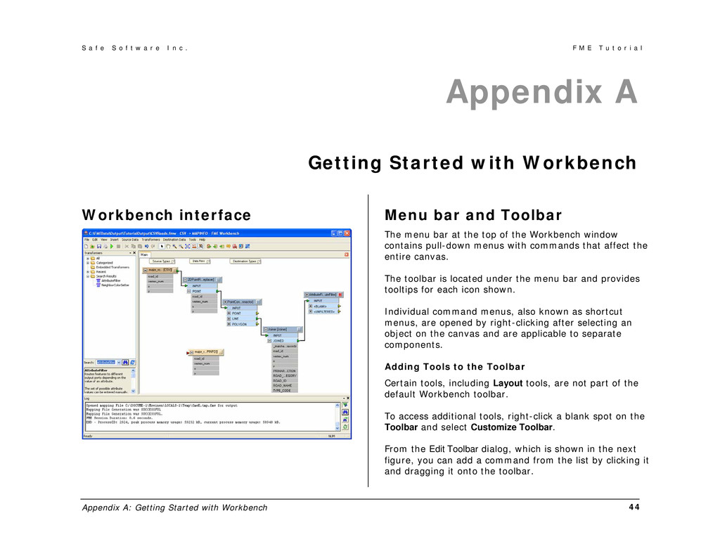
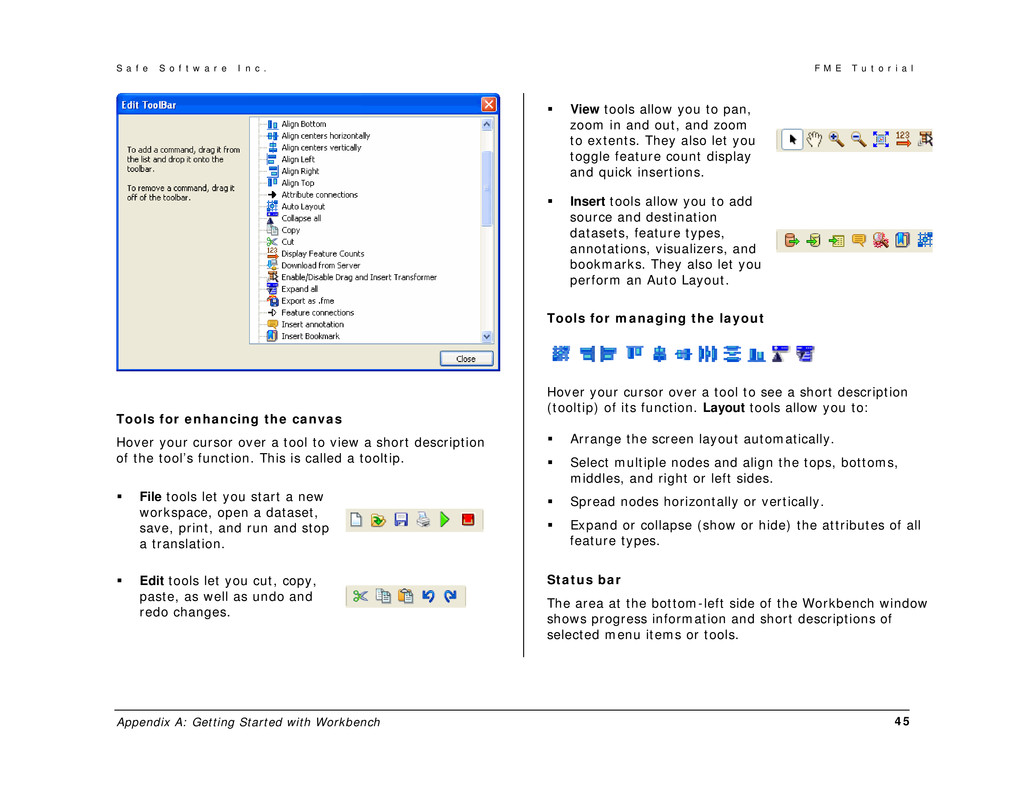
r e I n c . F M E T u t o r i a l Appendix A: Getting Started with Workbench 44 Appendix A Getting Started with Workbench Workbench interface Menu bar and Toolbar The menu bar at the top of the Workbench window contains pull-down menus with commands that affect the entire canvas. The toolbar is located under the menu bar and provides tooltips for each icon shown. Individual command menus, also known as shortcut menus, are opened by right-clicking after selecting an object on the canvas and are applicable to separate components. Adding Tools to the Toolbar Certain tools, including Layout tools, are not part of the default Workbench toolbar. To access additional tools, right-click a blank spot on the Toolbar and select Customize Toolbar. From the Edit Toolbar dialog, which is shown in the next figure, you can add a command from the list by clicking it and dragging it onto the toolbar.
r e I n c . F M E T u t o r i a l Appendix A: Getting Started with Workbench 45 Tools for enhancing the canvas Hover your cursor over a tool to view a short description of the tool’s function. This is called a tooltip. File tools let you start a new workspace, open a dataset, save, print, and run and stop a translation. Edit tools let you cut, copy, paste, as well as undo and redo changes. View tools allow you to pan, zoom in and out, and zoom to extents. They also let you toggle feature count display and quick insertions. Insert tools allow you to add source and destination datasets, feature types, annotations, visualizers, and bookmarks. They also let you perform an Auto Layout. Tools for managing the layout Hover your cursor over a tool to see a short description (tooltip) of its function. Layout tools allow you to: Arrange the screen layout automatically. Select multiple nodes and align the tops, bottoms, middles, and right or left sides. Spread nodes horizontally or vertically. Expand or collapse (show or hide) the attributes of all feature types. Status bar The area at the bottom-left side of the Workbench window shows progress information and short descriptions of selected menu items or tools.
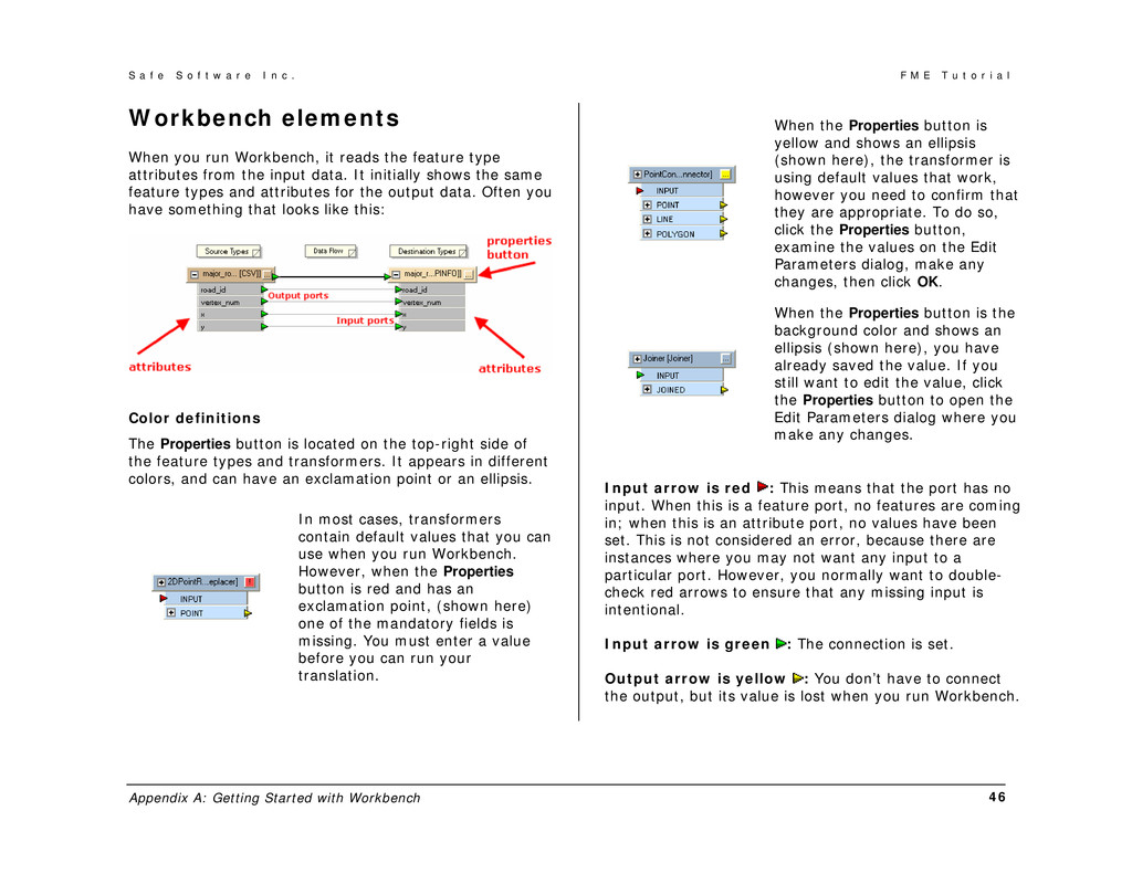
r e I n c . F M E T u t o r i a l Appendix A: Getting Started with Workbench 46 Workbench elements When you run Workbench, it reads the feature type attributes from the input data. It initially shows the same feature types and attributes for the output data. Often you have something that looks like this: Color definitions The Properties button is located on the top-right side of the feature types and transformers. It appears in different colors, and can have an exclamation point or an ellipsis. In most cases, transformers contain default values that you can use when you run Workbench. However, when the Properties button is red and has an exclamation point, (shown here) one of the mandatory fields is missing. You must enter a value before you can run your translation. When the Properties button is yellow and shows an ellipsis (shown here), the transformer is using default values that work, however you need to confirm that they are appropriate. To do so, click the Properties button, examine the values on the Edit Parameters dialog, make any changes, then click OK. When the Properties button is the background color and shows an ellipsis (shown here), you have already saved the value. If you still want to edit the value, click the Properties button to open the Edit Parameters dialog where you make any changes. Input arrow is red : This means that the port has no input. When this is a feature port, no features are coming in; when this is an attribute port, no values have been set. This is not considered an error, because there are instances where you may not want any input to a particular port. However, you normally want to double- check red arrows to ensure that any missing input is intentional. Input arrow is green : The connection is set. Output arrow is yellow : You don’t have to connect the output, but its value is lost when you run Workbench.
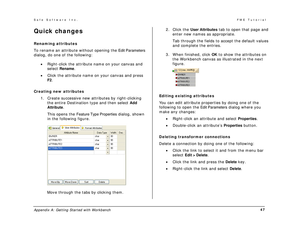
r e I n c . F M E T u t o r i a l Appendix A: Getting Started with Workbench 47 Quick changes Renaming attributes To rename an attribute without opening the Edit Parameters dialog, do one of the following: • Right-click the attribute name on your canvas and select Rename. • Click the attribute name on your canvas and press F2. Creating new attributes 1. Create successive new attributes by right-clicking the entire Destination type and then select Add Attribute. This opens the Feature Type Properties dialog, shown in the following figure. Move through the tabs by clicking them. 2. Click the User Attributes tab to open that page and enter new names as appropriate. Tab through the fields to accept the default values and complete the entries. 3. When finished, click OK to show the attributes on the Workbench canvas as illustrated in the next figure. Editing existing attributes You can edit attribute properties by doing one of the following to open the Edit Parameters dialog where you make any changes: • Right-click an attribute and select Properties. • Double-click an attribute’s Properties button. Deleting transformer connections Delete a connection by doing one of the following: • Click the link to select it and from the menu bar select Edit > Delete. • Click the link and press the Delete key. • Right-click the link and select Delete.
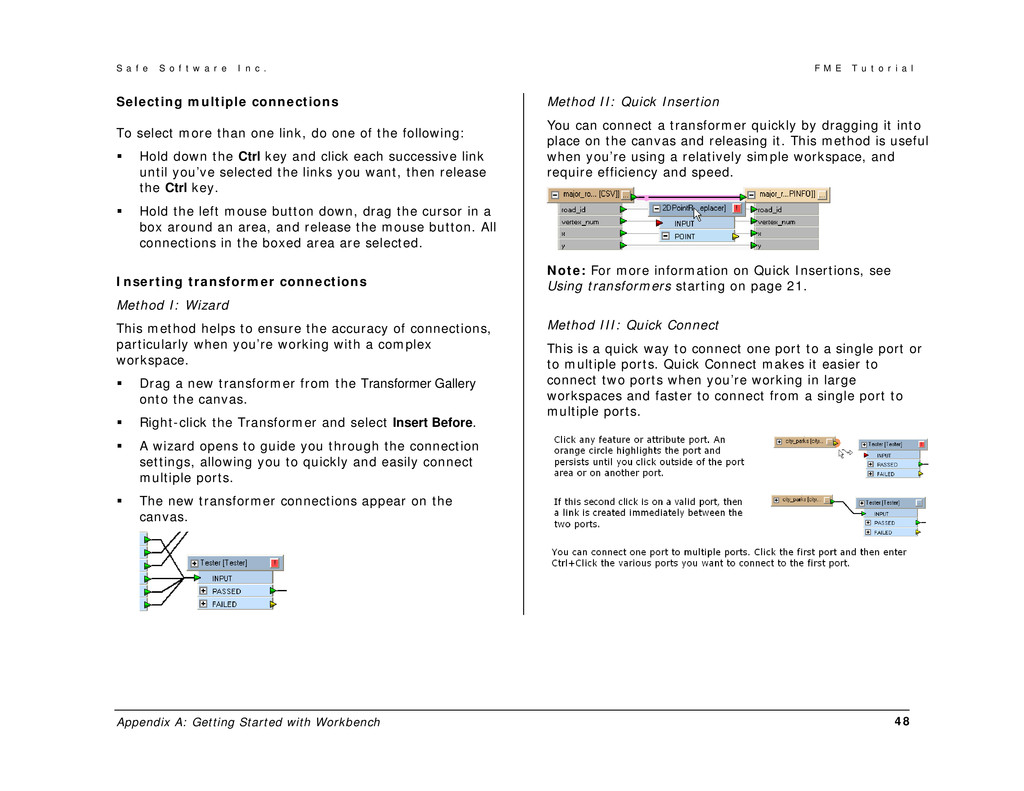
r e I n c . F M E T u t o r i a l Appendix A: Getting Started with Workbench 48 Selecting multiple connections To select more than one link, do one of the following: Hold down the Ctrl key and click each successive link until you’ve selected the links you want, then release the Ctrl key. Hold the left mouse button down, drag the cursor in a box around an area, and release the mouse button. All connections in the boxed area are selected. Inserting transformer connections Method I: Wizard This method helps to ensure the accuracy of connections, particularly when you’re working with a complex workspace. Drag a new transformer from the Transformer Gallery onto the canvas. Right-click the Transformer and select Insert Before. A wizard opens to guide you through the connection settings, allowing you to quickly and easily connect multiple ports. The new transformer connections appear on the canvas. Method II: Quick Insertion You can connect a transformer quickly by dragging it into place on the canvas and releasing it. This method is useful when you’re using a relatively simple workspace, and require efficiency and speed. Note: For more information on Quick Insertions, see Using transformers starting on page 21. Method III: Quick Connect This is a quick way to connect one port to a single port or to multiple ports. Quick Connect makes it easier to connect two ports when you’re working in large workspaces and faster to connect from a single port to multiple ports.
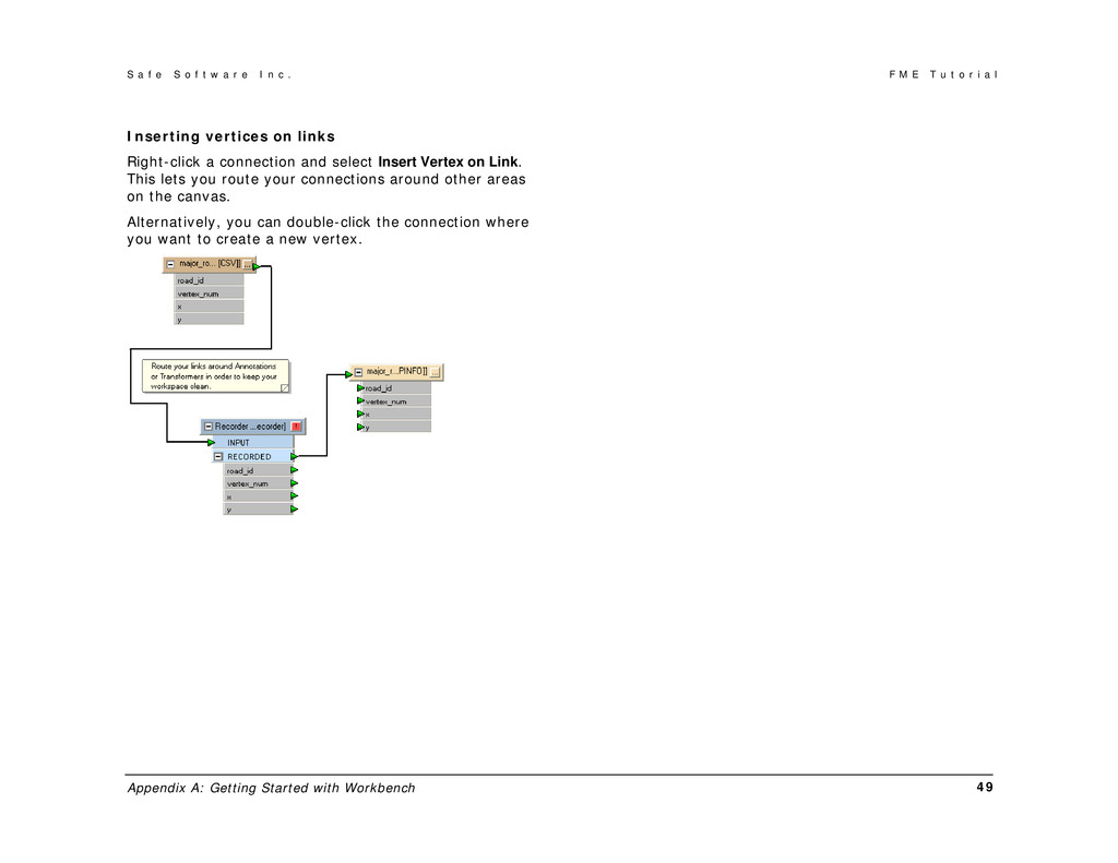
r e I n c . F M E T u t o r i a l Appendix A: Getting Started with Workbench 49 Inserting vertices on links Right-click a connection and select Insert Vertex on Link. This lets you route your connections around other areas on the canvas. Alternatively, you can double-click the connection where you want to create a new vertex.