Digitizing Polygons using QGIS

Digitizing and Cleaning up Polygons using QGIS
http://www.netconstructor.com

Transcript

1. Perfect Polygons in QGIS The Polygonizer Plug-in 1
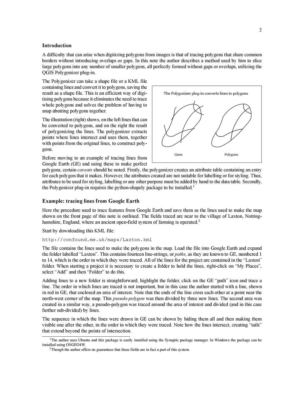
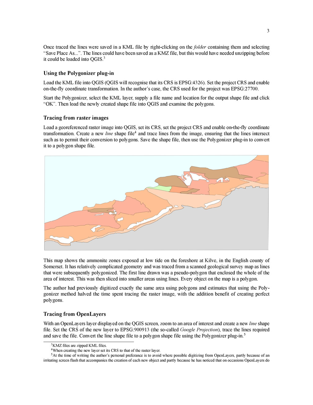
2. 2 Introduction A difficulty that can arise when digitizing polygons from images is that of tracing polygons that share common borders without introducing overlaps or gaps. In this note the author describes a method used by him to slice large polygons into any number of smaller polygons, all perfectly formed without gaps or overlaps, utilizing the QGIS Polygonizer plug-in. Lines Polygons The Polygonizer plug-in converts lines to polygons The Polygonizer can take a shape file or a KML file containing lines and convert it to polygons, saving the result as a shape file. This is an efficient way of digi- tising polygons because it eliminates the need to trace whole polygons and solves the problem of having to snap abutting polygons together. The illustration (right) shows, on the left lines that can be converted to polygons, and on the right the result of polygonizing the lines. The polygonizer extracts points where lines intersect and uses them, together with points from the original lines, to construct poly- gons. Before moving to an example of tracing lines from Google Earth (GE) and using these to make perfect polygons, certain caveats should be noted. Firstly, the polygonizer creates an attribute table containing an entry for each polygon that it makes. However, the attributes created are not suitable for labelling or for styling. Thus, attributes to be used for styling, labelling or any other purpose must be added by hand to the data table. Secondly, the Polygonizer plug-in requires the python-shapely package to be installed.1 Example: tracing lines from Google Earth Here the procedure used to trace features from Google Earth and save them as the lines used to make the map shown on the front page of this note is outlined. The fields traced are near to the village of Laxton, Notting- hamshire, England, where an ancient open-field system of farming is operated.2 Start by downloading this KML file: http://confound.me.uk/maps/Laxton.kml The file contains the lines used to make the polygons in the map. Load the file into Google Earth and expand the folder labelled “Laxton”. This contains fourteen line-strings, or paths, as they are known to GE, numbered 1 to 14, which is the order in which they were traced. All of the lines for the project are contained in the “Laxton” folder. When starting a project it is necessary to create a folder to hold the lines, right-click on “My Places”, select “Add” and then “Folder” to do this. Adding lines to a new folder is straightforward, highlight the folder, click on the GE “path” icon and trace a line. The order in which lines are traced is not important, but in this case the author started with a line, shown in red in GE, that enclosed an area of interest. Note that the ends of the line cross each other at a point near the north-west corner of the map. This pseudo-polygon was then divided by three new lines. The second area was created in a similar way, a pseudo-polygon was traced around the area of interest and divided (and in this case further sub-divided) by lines. The sequence in which the lines were drawn in GE can be shown by hiding them all and then making them visible one after the other, in the order in which they were traced. Note how the lines intersect, creating “tails” that extend beyond the points of intersection. 1The author uses Ubuntu and this package is easily installed using the Synaptic package manager. In Windows the package can be installed using OSGEO4W. 2Though the author offers no guarantees that these fields are in fact a part of this system.
3. 3 Once traced the lines were saved in a KML file by right-clicking on the folder containing them and selecting “Save Place As...”. The lines could have been saved as a KMZ file, but this would have needed unzipping before it could be loaded into QGIS.3 Using the Polygonizer plug-in Load the KML file into QGIS (QGIS will recognise that its CRS is EPSG:4326). Set the project CRS and enable on-the-fly coordinate transformation. In the author’s case, the CRS used for the project was EPSG:27700. Start the Polygonizer, select the KML layer, supply a file name and location for the output shape file and click “OK”. Then load the newly created shape file into QGIS and examine the polygons. Tracing from raster images Load a georeferenced raster image into QGIS, set its CRS, set the project CRS and enable on-the-fly coordinate transformation. Create a new line shape file4 and trace lines from the image, ensuring that the lines intersect such as to permit their conversion to polygons. Save the shape file, then use the Polygonizer plug-in to convert it to a polygon shape file. This map shows the ammonite zones exposed at low tide on the foreshore at Kilve, in the English county of Somerset. It has relatively complicated geometry and was traced from a scanned geological survey map as lines that were subsequently polygonized. The first line drawn was a pseudo-polygon that enclosed the whole of the area of interest. This was then sliced into smaller areas using lines. Every object on the map is a polygon. The author had previously digitized exactly the same area using polygons and estimates that using the Poly- gonizer method halved the time spent tracing the raster image, with the addition benefit of creating perfect polygons. Tracing from OpenLayers With an OpenLayers layer displayed on the QGIS screen, zoom to an area of interest and create a new line shape file. Set the CRS of the new layer to EPSG:900913 (the so-called Google Projection), trace the lines required and save the file. Convert the line shape file to a polygon shape file using the Polygonizer plug-in.5 3KMZ files are zipped KML files. 4When creating the new layer set its CRS to that of the raster layer. 5At the time of writing the author’s personal preferance is to avoid where possible digitizing from OpenLayers, partly because of an irritating screen flash that accompanies the creation of each new object and partly because he has noticed that on occasions OpenLayers do
4. 4 Styling As mentioned earlier, the polygonizer creates an attribute table containing an entry for each polygon in the shape file. The attributes, however, are of no use for labelling or styling. The map shown on the front page of this note was styled using attributes added to a new column in the data table. In this case the attributes were sequential numbers entered using the field calculator. Acknowledgements The Polygonizer plug-in is the creation of Piotr Pociask and his efforts on behalf of the QGIS community are gratefully acknowledged. About the author The author of this note is Nick Hopton. Comments on the note may be addressed to nhopton@gmail.com. not register correctly on the QGIS screen.