Creating Population Surfaces for the Analysis of Small Area Change

Presented at British Society for Population Studies at University of Leeds on 7th September 2015

Transcript

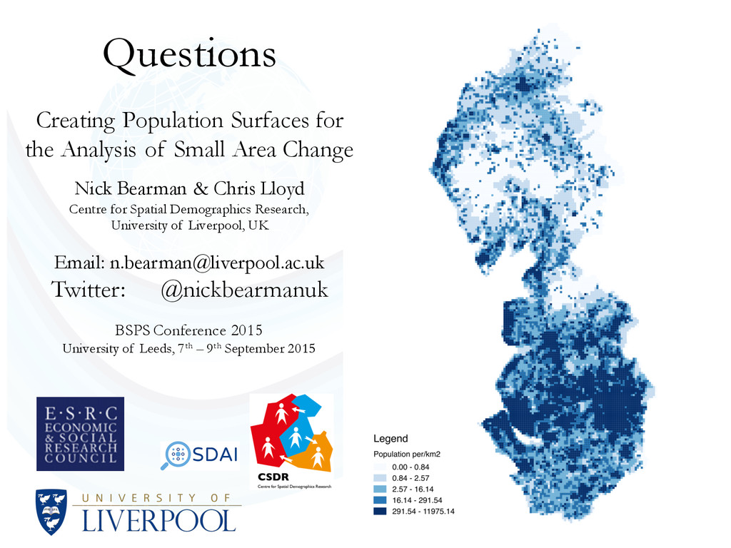
1. Creating Population Surfaces for the Analysis of Small Area Change Nick Bearman & Chris Lloyd Centre for Spatial Demographics Research, University of Liverpool, UK Email: n.bearman@liverpool.ac.uk Twitter: @nickbearmanuk BSPS Conference 2015, University of Leeds, 7th – 9th September 2015
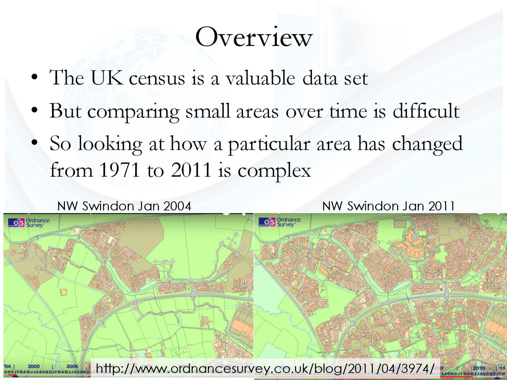
2. Overview • The UK census is a valuable data set • But comparing small areas over time is difficult • So looking at how a particular area has changed from 1971 to 2011 is complex NW Swindon Jan 2004 NW Swindon Jan 2011 http://www.ordnancesurvey.co.uk/blog/2011/04/3974/
3. Overview Three main problems: 1. Size and shape of the zones used 2. Questions asked 3. Output variables ecimen Individual questions - Person 1 start here Married Separated, but still legally married Divorced Widowed What is your name? (Person 1 on page 3) First name Last name What is your sex? Male Female What is your date of birth? Are you a schoolchild or student in full-time education? Yes No During term time, do you live: at the address on the front of this questionnaire? at the address in question 5? at another address? What is your country of birth? England Wales Scotland Northern Ireland Republic of Ireland Elsewhere, write in the current name of country If you were not born in the United Kingdom, when did you most recently arrive to live here? Do not count short visits away from the UK Including the time you have already spent here, how long do you intend to stay in the United Kingdom? Do you stay at another address for more than 30 days a year? No Yes, write in other UK address below On 27 March 2011, what is your legal marital or same-sex civil partnership status? Never married and never registered a same-sex civil partnership In a registered same-sex civil partnership Separated, but still legally in a same-sex civil partnership Formerly in a same-sex civil partnership which is now legally dissolved Surviving partner from a same-sex civil partnership If you arrived before 27 March 2010 If you arrived on or after 27 March 2010 1 2 3 7 8 9 11 4 10 5 12 Go to 13 Go to 7 Go to 43 Go to 9 Go to 43 Go to 13 Go to 13 Go to 13 Go to 13 Go to 12 Day Month Year Month Year
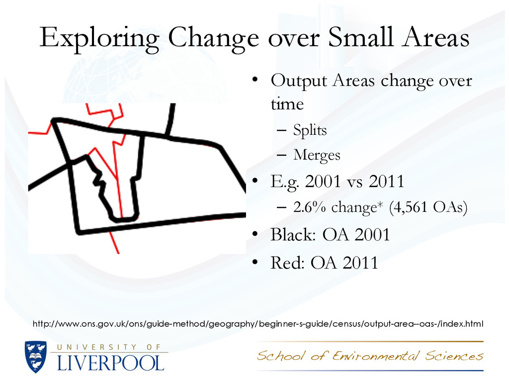
4. Exploring Change over Small Areas • Output Areas change over time – Splits – Merges • E.g. 2001 vs 2011 – 2.6% change* (4,561 OAs) • Black: OA 2001 • Red: OA 2011 http://www.ons.gov.uk/ons/guide-method/geography/beginner-s-guide/census/output-area--oas-/index.html
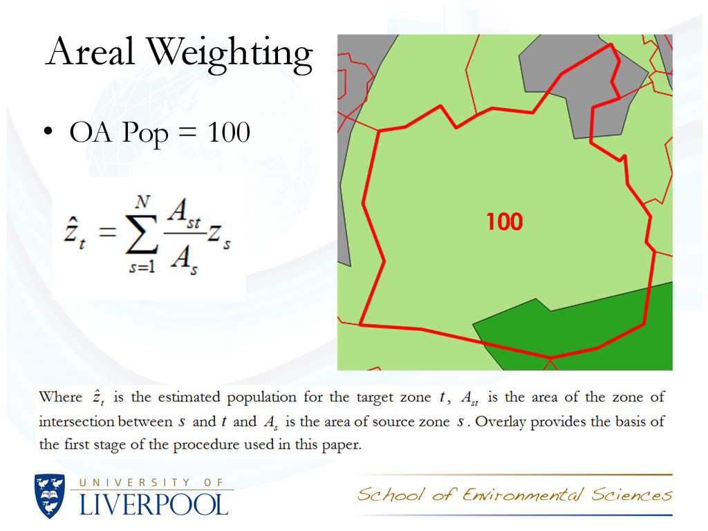
5. Exploring Change over Small Areas Solutions to the first problem include: (i) converting counts from irregular zones to a surface (ii) transferring counts from one set of zones to another using areal interpolation (iii)transferring counts from one set of zones to another on a best-fit basis (Martin et al., 2002). This research focuses on a combination of (i) and (ii).
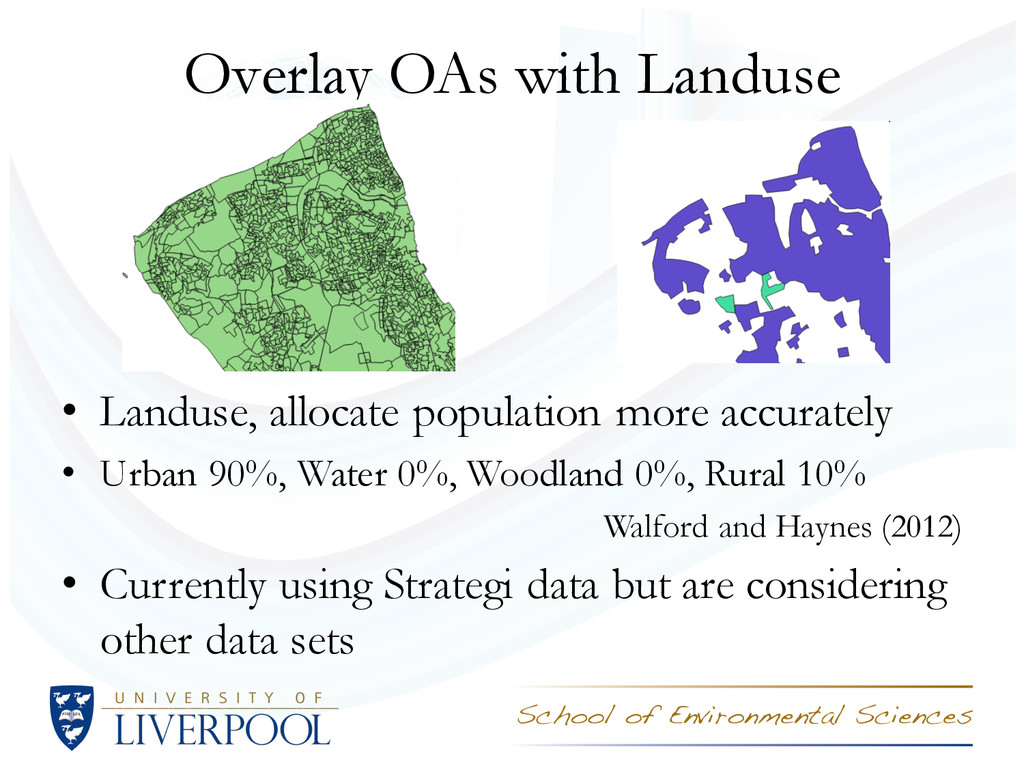
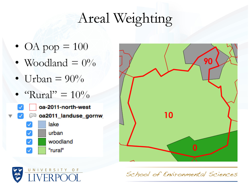
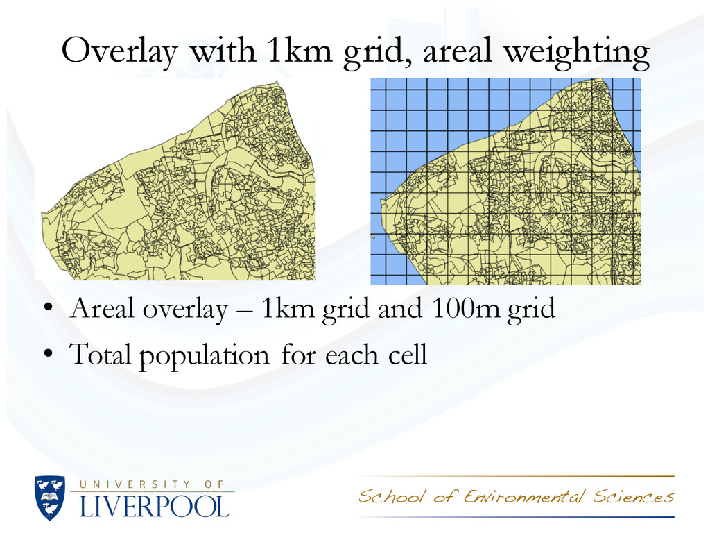
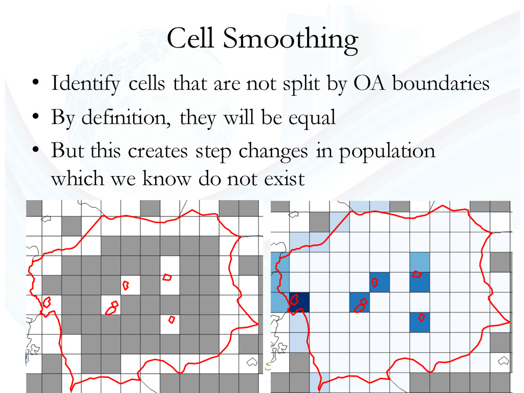
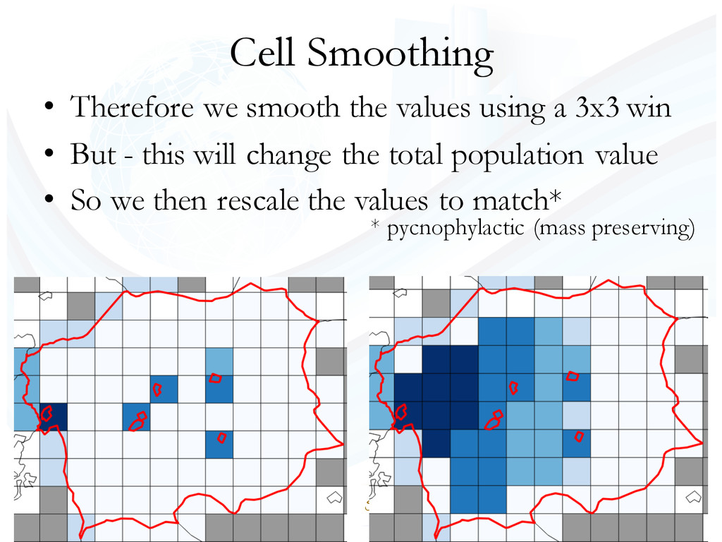
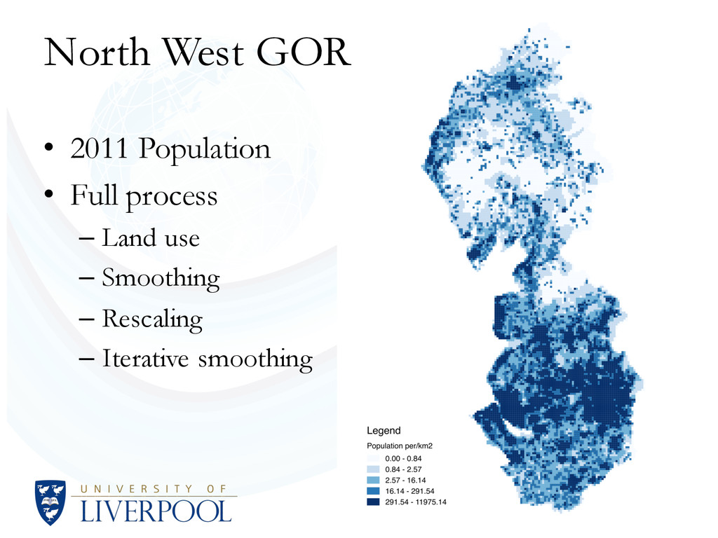
6. The Process • Identify comparable variables • Overlay OAs (EDs) with landuse data • Use areal overlay & weighting to estimate population • Overlay 1km grid (100m urban) • Use areal overlay & weighting with grid & OA • Smooth grid cells
7. Overlay OAs with Landuse • Landuse, allocate population more accurately • Urban 90%, Water 0%, Woodland 0%, Rural 10% Walford and Haynes (2012) • Currently using Strategi data but are considering other data sets
8. Areal Weighting • OA Pop = 100 100
9. Areal Weighting • OA pop = 100 • Woodland = 0% • Urban = 90% • “Rural” = 10% 10 0 90
10. Overlay with 1km grid, areal weighting • Areal overlay – 1km grid and 100m grid • Total population for each cell
11. Cell Smoothing • Identify cells that are not split by OA boundaries • By definition, they will be equal • But this creates step changes in population which we know do not exist
12. Cell Smoothing • Therefore we smooth the values using a 3x3 win • But - this will change the total population value • So we then rescale the values to match* * pycnophylactic (mass preserving)
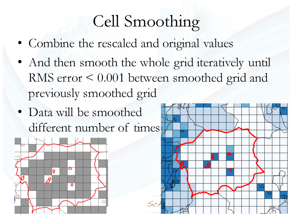
13. Cell Smoothing • Combine the rescaled and original values • And then smooth the whole grid iteratively until RMS error < 0.001 between smoothed grid and previously smoothed grid • Data will be smoothed different number of times
14. Cell Smoothing The number (n) of smoothing iterations for each count until the RMS difference decreased to less than 0.001. 2001 2011 Counts n iterations n iterations White 16 11 Non-White 3 3 LLTI 10 7 No LLTI 15 10 The figures accord with expectation in that a larger number of iterations is required to reach convergence for ‘smoother’ counts than is the case for less-smooth counts. The categories White and No LLTI each include the large majority of people and are relatively spatial homogenous compared the categories Non-White and LLTI. Therefore, more smoothing is likely to be optimal in the former cases than in the latter. Also, the results suggest that ‘White’ and ‘No LLTI’ were, on average, smoother in 2001 than they were in 2011.
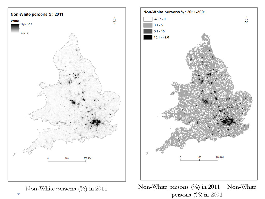
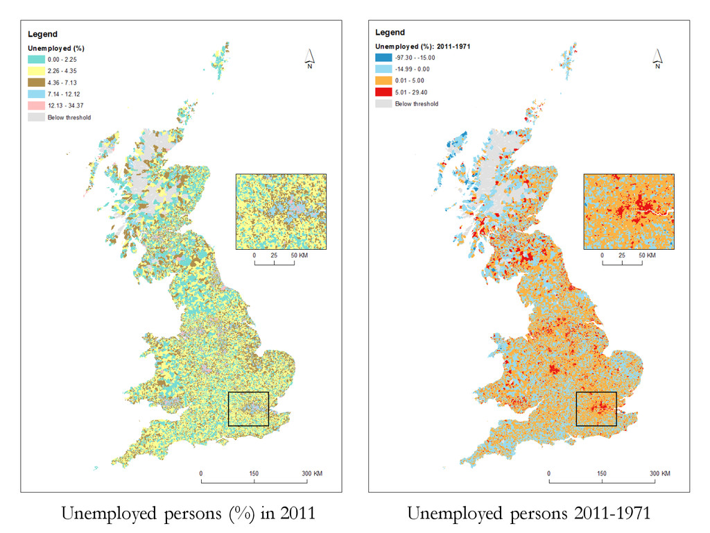
15. Provisional Results: 1971, 2001 & 2011 • Data for 1971 (EDs) and 2011 (OAs) have been reallocated to 1km grids for Britain (no land use data or smoothing) • Derived variables include: - Ethnicity, England & Wales (2011 – 2001) - Limiting Long Term Illness, E & W (2011 – 2011) - Unemployed persons, E, W & S (% of unemployed, 2011 – 1971) -Population Count, North West GOR
16. Non-White persons (%) in 2011 – Non-White persons (%) in 2001 Non-White persons (%) in 2011
17. Persons with a LLTI (%) in 2011 Persons with a LLTI (%) in 2011 – persons with a LLTI (%) in 2001
18. Unemployed persons (%) in 2011 Unemployed persons 2011-1971
19. • 2011 Population • Full process – Land use – Smoothing – Rescaling – Iterative smoothing North West GOR
20. Data & Code • Data will be available online and stored with the UK Data Service • Code written in R • Code will be made available through GitHub • We welcome your comments, contributions and improvements! • Presentation is available online () – & code will be soon!
21. Summary • Areal reallocation of data rather than just centroids • Combination with ancillary data (landuse) and smoothing makes the most of the available data • Required iterations smoothing varies • 1km2 grid squares for UK, 100m2 for urban areas • Can apply to a set of variables for each Census from 1971 to 2011 for the whole of the UK
22. Acknowledgements Support from the ESRC is acknowledged gratefully (Grant Ref No ES/L014769/1). Team members also include Gemma Catney, Alex Singleton and Paul Williamson. The Office for National Statistics are thanked for provision of the data. Office for National Statistics, 2011 Census: Digitised Boundary Data (England and Wales) [computer file]. ESRC/JISC Census Programme, Census Geography Data Unit (UKBORDERS), EDINA (University of Edinburgh)/Census Dissemination Unit. Census output is Crown copyright and is reproduced with the permission of the Controller of HMSO and the Queen's Printer for Scotland.
23. Questions Creating Population Surfaces for the Analysis of Small Area Change Nick Bearman & Chris Lloyd Centre for Spatial Demographics Research, University of Liverpool, UK Email: n.bearman@liverpool.ac.uk Twitter: @nickbearmanuk BSPS Conference 2015 University of Leeds, 7th – 9th September 2015