Department of Geography and Planning TravelOAC: development of travel geodemographic classifica9ons for England and Wales based on open data TwiBer: @nickbearmanuk "Cyclists at red 2" by heb@Wikimedia Commons (mail) -‐ Own work. Licensed under CC BY-‐SA 3.0 via Wikimedia Commons -‐ hBp://commons.wikimedia.org/ wiki/File:Cyclists_at_red_2.jpg#/media/File:Cyclists_at_red_2.jpg epSos.de, hBps://www.flickr.com/photos/epsos/5591761716/
different factors influence our choice of method of travel • Travel choice is important – CO2 emissions – Conges^on – Cost / Time – Availability – Infrastructure development • This analysis is possible due to big data analysis and 2011 Census "High Five Interchange". Licensed under CC BY 2.0 via Wikimedia Commons -‐ hBp://commons.wikimedia.org/wiki/ File:High_Five_Interchange.jpg#/media/File:High_Five_Interchange.jpg
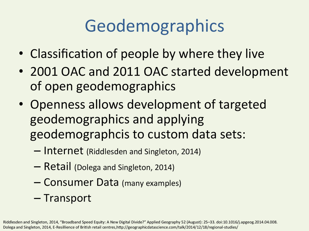
• 2001 OAC and 2011 OAC started development of open geodemographics • Openness allows development of targeted geodemographics and applying geodemographcis to custom data sets: – Internet (Riddlesden and Singleton, 2014) – Retail (Dolega and Singleton, 2014) – Consumer Data (many examples) – Transport Riddlesden and Singleton, 2014, “Broadband Speed Equity: A New Digital Divide?” Applied Geography 52 (August): 25–33. doi:10.1016/j.apgeog.2014.04.008. Dolega and Singleton, 2014, E-‐Resillience of Bri^sh retail centres,hBp://geographicdatascience.com/talk/2014/12/18/regional-‐studies/
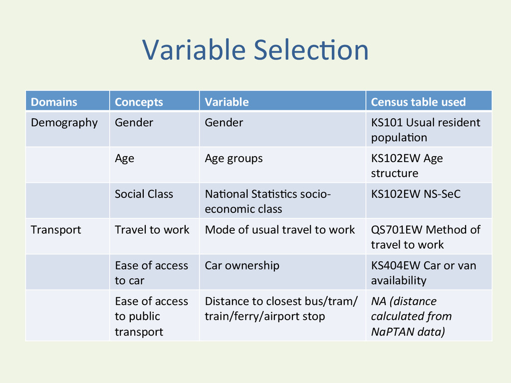
table used Demography Gender Gender KS101 Usual resident popula^on Age Age groups KS102EW Age structure Social Class Na^onal Sta^s^cs socio-‐ economic class KS102EW NS-‐SeC Transport Travel to work Mode of usual travel to work QS701EW Method of travel to work Ease of access to car Car ownership KS404EW Car or van availability Ease of access to public transport Distance to closest bus/tram/ train/ferry/airport stop NA (distance calculated from NaPTAN data)
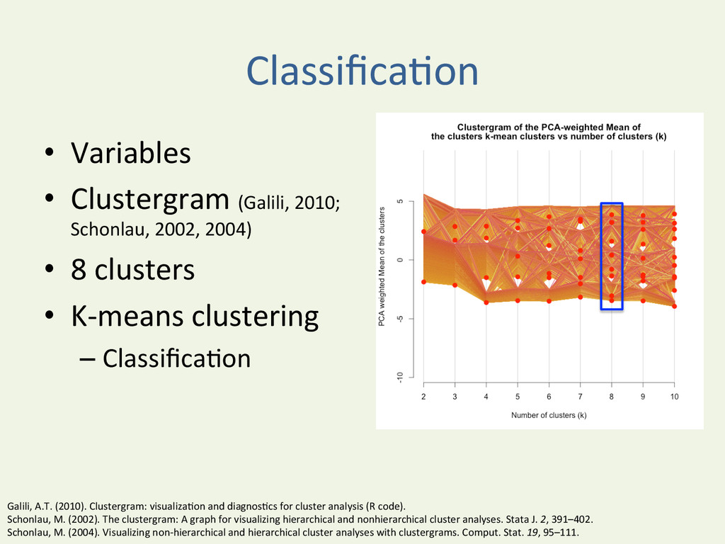
Schonlau, 2002, 2004) • 8 clusters • K-‐means clustering – Classifica^on Galili, A.T. (2010). Clustergram: visualiza^on and diagnos^cs for cluster analysis (R code). Schonlau, M. (2002). The clustergram: A graph for visualizing hierarchical and nonhierarchical cluster analyses. Stata J. 2, 391–402. Schonlau, M. (2004). Visualizing non-‐hierarchical and hierarchical cluster analyses with clustergrams. Comput. Stat. 19, 95–111.
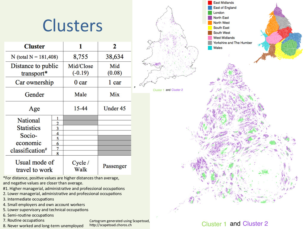
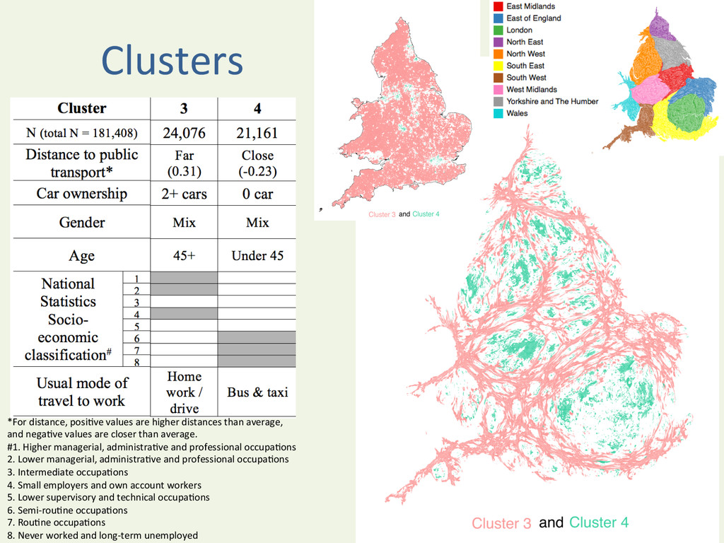
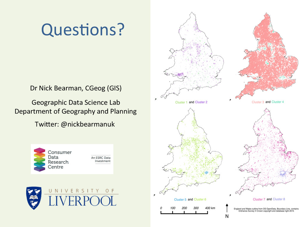
and nega^ve values are closer than average. #1. Higher managerial, administra^ve and professional occupa^ons 2. Lower managerial, administra^ve and professional occupa^ons 3. Intermediate occupa^ons 4. Small employers and own account workers 5. Lower supervisory and technical occupa^ons 6. Semi-‐rou^ne occupa^ons 7. Rou^ne occupa^ons 8. Never worked and long-‐term unemployed • Cartogram generated using Scapetoad, hBp://scapetoad.choros.ch Clusters
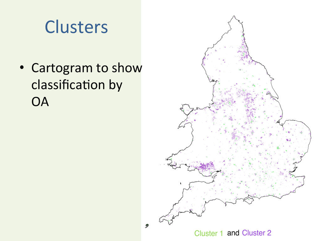
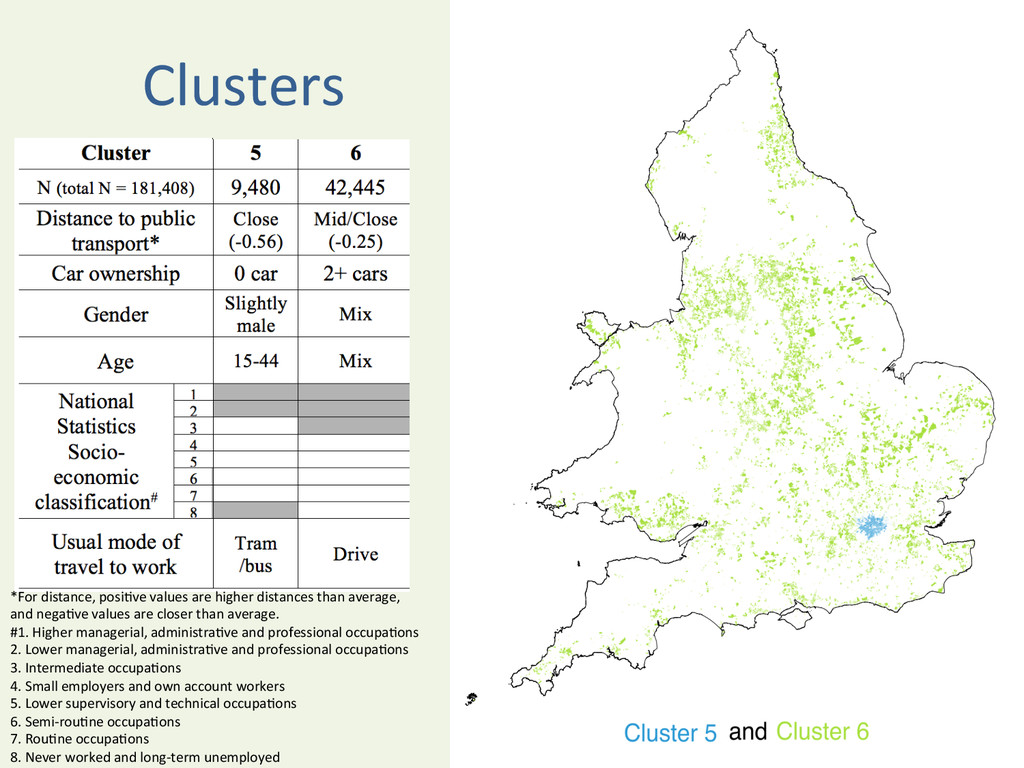
and nega^ve values are closer than average. #1. Higher managerial, administra^ve and professional occupa^ons 2. Lower managerial, administra^ve and professional occupa^ons 3. Intermediate occupa^ons 4. Small employers and own account workers 5. Lower supervisory and technical occupa^ons 6. Semi-‐rou^ne occupa^ons 7. Rou^ne occupa^ons 8. Never worked and long-‐term unemployed Clusters
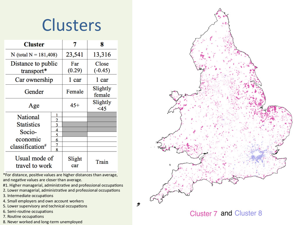
and nega^ve values are closer than average. #1. Higher managerial, administra^ve and professional occupa^ons 2. Lower managerial, administra^ve and professional occupa^ons 3. Intermediate occupa^ons 4. Small employers and own account workers 5. Lower supervisory and technical occupa^ons 6. Semi-‐rou^ne occupa^ons 7. Rou^ne occupa^ons 8. Never worked and long-‐term unemployed Clusters
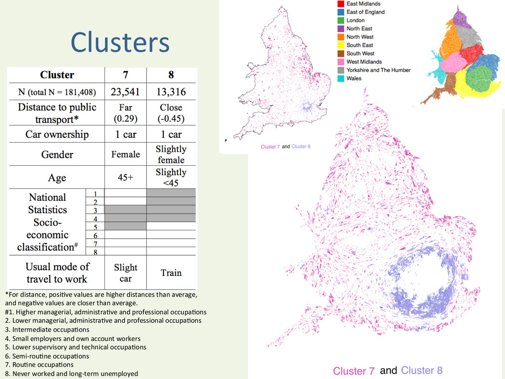
and nega^ve values are closer than average. #1. Higher managerial, administra^ve and professional occupa^ons 2. Lower managerial, administra^ve and professional occupa^ons 3. Intermediate occupa^ons 4. Small employers and own account workers 5. Lower supervisory and technical occupa^ons 6. Semi-‐rou^ne occupa^ons 7. Rou^ne occupa^ons 8. Never worked and long-‐term unemployed Clusters
and nega^ve values are closer than average. #1. Higher managerial, administra^ve and professional occupa^ons 2. Lower managerial, administra^ve and professional occupa^ons 3. Intermediate occupa^ons 4. Small employers and own account workers 5. Lower supervisory and technical occupa^ons 6. Semi-‐rou^ne occupa^ons 7. Rou^ne occupa^ons 8. Never worked and long-‐term unemployed Clusters
and nega^ve values are closer than average. #1. Higher managerial, administra^ve and professional occupa^ons 2. Lower managerial, administra^ve and professional occupa^ons 3. Intermediate occupa^ons 4. Small employers and own account workers 5. Lower supervisory and technical occupa^ons 6. Semi-‐rou^ne occupa^ons 7. Rou^ne occupa^ons 8. Never worked and long-‐term unemployed Clusters
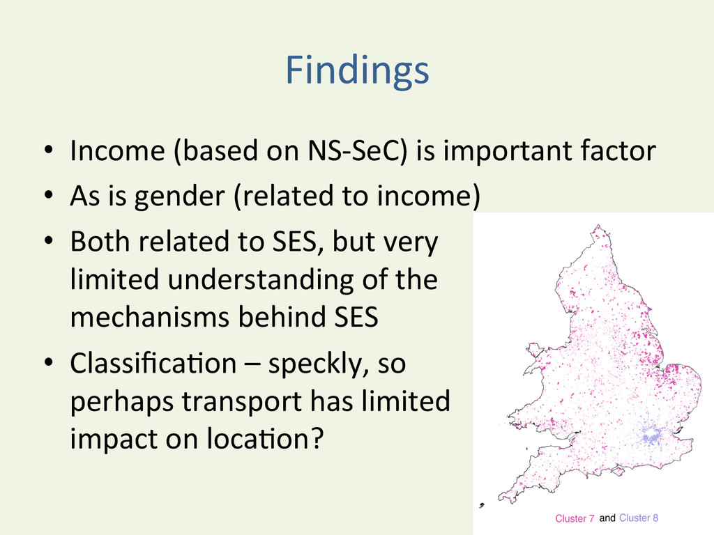
average, and nega^ve values are closer than average. #1. Higher managerial, administra^ve and professional occupa^ons 2. Lower managerial, administra^ve and professional occupa^ons 3. Intermediate occupa^ons 4. Small employers and own account workers 5. Lower supervisory and technical occupa^ons 6. Semi-‐rou^ne occupa^ons 7. Rou^ne occupa^ons 8. Never worked and long-‐term unemployed
• As is gender (related to income) • Both related to SES, but very limited understanding of the mechanisms behind SES • Classifica^on – speckly, so perhaps transport has limited impact on loca^on?
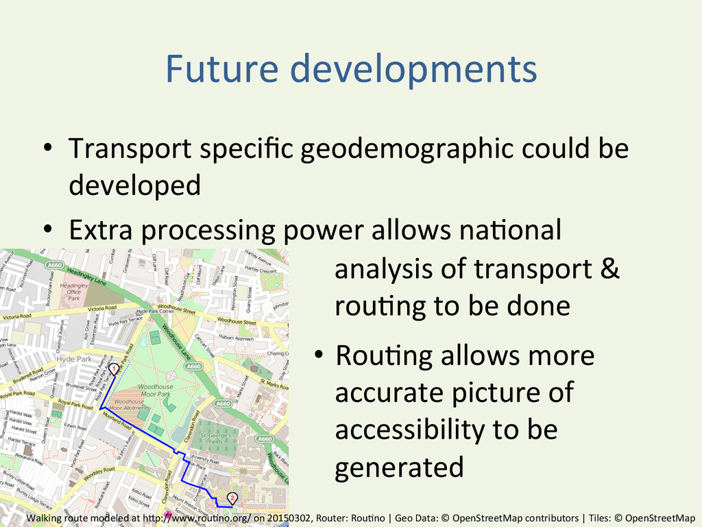
use and access • Do the two factors match? • Jus^fica^on for development of new sta^ons / services • Applica^on could be applied to more refined data (e.g. ^cket sales, usage surveys, etc.) s^ll using the rou^ng element "KingsCrossDevelopmentModel". Licensed under CC BY-‐SA 2.0 via Wikimedia Commons -‐ hBp://commons.wikimedia.org/wiki/ File:KingsCrossDevelopmentModel.jpg#/media/ File:KingsCrossDevelopmentModel.jpg