A series of reviews related to kumamoto earthquake(2016)

Transcript

1. Review : Method for estimating the stress field from seismic moment tensor data based on the flow rule in plasticity theory (Matsumoto, 2016) Prestate of Stress and Fault Behavior During the 2016 Kumamoto Earthquake (M7.3) (Matsumoto et al., 2018)
2. Overall Matsumoto(2016) Matsumoto et al. (2018) • Develop SMT method the inversion method to estimate a stress field • (Compare with existing method) • Apply the method to Kyusyu • Discuss the coseismic rupture in Kumamoto earthquake(2016) • Discuss the pore fluid pressure and the subsurface structure
3. What did they do? (Matsumoto, 2016) • Develop the inversion method for estimating the stress field • Prove : • What we can : Stress ratio and Principal stress directions are estimated by the sum of moment tensors • Limitation • Test the method for shallow earthquakes occurring on Kyushu k : k-th earthquake
4. Estimate the stress field Formula about moment tensor (Noda and Matsu'ura, 2010) m : moment density tensor τ : model stress σ : physical stress C : compliance εa : inelastic strain εe : elastic strain Next, assume εa (inelastic strain) as εp(plastic strain)
5. Estimate the stress field Prove that Deviatoric stress tensor ∝ Moment density tensor Prandtl-Reuss formula : Formula about moment tensor: assume isotropic s : deviatoric stress tensor dλ : positive scalar value = the plastic strain and deviatoric stress tensor have the same principal directions μ : rigidity
6. Estimate the stress field the sum of the moment tensors -> estimate Stress ratio and Principal stress directions s : deviatoric stress tensor dλ : positive scalar value μ : Lamé's constants m : moment density tensor Mk : total moment tensor released in a k-th earthquake ΔV : the area affected by earthquakes introduce the flow rule in plasticity and Kostrov's sum Kostrov's sum (Kostrov, 1974) assuming a uniform seismic moment density
7. Estimate the stress field Limitation of this method (call SMT method) ✖ evaluate the proportionality coefficient unable to estimate absolute values of stress tensor ✖ single large event and small events because it assumes homogenous moment density tensor distribution ✖ contains weak faults because the stress field might be heterogeneous in the volume
8. What did they do? (Matsumoto, 2016) • Develop the inversion method for estimating the stress field • Prove : Deviatoric stress tensor ∝ Moment density tensor • What we can : Stress ratio and Principal stress directions are estimated by the sum of moment tensors • Limitation • Test the method for shallow earthquakes occurring on Kyushu
9. Data Shallow earthquakes occurred in Kyusyu - 2000/01 – 2013/07 - magnitude > 1.0 - depth 0 – 30 km
10. Result
11. Compare SMT method with SATSI method What is SATSI method(Hardebeck and Michael, 2006)? • It is the application of Michael(1984) . • It estimates the spatial variation of the stress field.
12. SATSI method is the application of Michael(1984) method What is Michael(1984) method ? calc Least-squares solution model param : stress tensor data : slip vector Kernel : fault normal vector of each focal mechanism Consider only misfit
13. What is SATSI method ? Consider both misfit and model length mij dij Gij : parameter of each grid calc damped least squares solution by introducing damping matrix
14. SMT method has good agreement with SATSI method (Hardebeck and Michael, 2006)
15. What did they do? (Matsumoto, 2018) • Estimate the stress field around Kumamoto earthquake faults • Lateral heterogeneous and depth-dependent stress fields were dominant when the earthquakes occured. • The earthquakes followed the prestate of stress. • Consider pre-condition of pore fluid pressure on the fault • Approximately 25% of the seismic moment release was from the weakest part (Δp > τmax) of the fault.
16. Estimate the stress field around faults Hinagu fault and Futagawa fault
17. Data • focal mechanism dataset stations : ＋ location : Kyusyu Island time : 1996/01 – 2016/04 (before Mj 6.5 earthquake) depth : 0 – 30 km magnitude : 1.5 – 4 • Determine focal mechanism of 2,403 events well fitted by HASH algorithm (Hardebeck and Shearer, 2002)
18. Principal stress distributions for 2,403 events P axis ｜ T axis ｜
19. Method and Validation • Method • SMT method; using • Grid size : 0.075°x 0.075°x 5 km (each contains more than 10 events) • Validation • Bootstrap resampling : calc 90% CI m : optimum tensor m’ : solution from the resampling dataset(within 90%)
20. Result : Stress tensor distributions • Horizontal heterogeneity • Vertical heterogeneity Why?
21. Discussion : Horizontal heterogeneity Futagawa fault σ1 ~ horizontal(strike-slip stress) σ1 ~ vertical(normal fault stress) regional difference of E-W compressional force
22. Discussion : Vertical heterogeneity shallower deeper Due to over burden pressure ? σ1 ~ horizontal σ1 ~ vertical
23. Result ：maximum shear stress direction on the fault (MAX-SSDF)
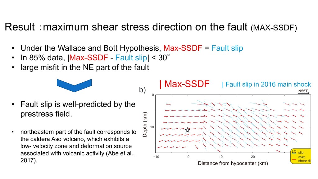
24. Result ：maximum shear stress direction on the fault (MAX-SSDF) • Under the Wallace and Bott Hypothesis, Max-SSDF = Fault slip • In 85% data, |Max-SSDF - Fault slip| < 30° • large misfit in the NE part of the fault | Max-SSDF • Fault slip is well-predicted by the prestress field. • northeastern part of the fault corresponds to the caldera Aso volcano, which exhibits a low- velocity zone and deformation source associated with volcanic activity (Abe et al., 2017). | Fault slip in 2016 main shock
25. What did they do? (Matsumoto, 2016) • Estimate the stress field around Kumamoto earthquake faults • Lateral heterogeneous and depth-dependent stress fields were dominant when the earthquakes occured. • The earthquakes followed the prestate of stress. • Consider pre-condition of pore fluid pressure on the fault • Heterogenity of pore fluid pressure • Approximately 25% of the seismic moment release was from the weakest part (Δp > τmax) of the fault.
26. Limitation of SMT method(again) SMT method can estimate only the direction of the principal stress axis and stress ratio = cannot estimate absolute value of the principal stress
27. Consider pre-condition of pore fluid pressure on the fault Calculate shear and normal stresses normalized by maximum shear stress Calculate Relative pore fluid pressure Δp’
28. Consider pre-condition of pore fluid pressure on the fault • Relative pore fluid pressure Δp’ distribution
29. Consider pre-condition of pore fluid pressure on the fault • Relative pore fluid pressure Δp’ distribution
30. Consider pre-condition of pore fluid pressure on the fault Δp’ (relative pore fluid pressure) fault orientation fault strength seismic moment high unfavorable weak low low favorable strong high Why is Δp’ (= Δp / τmax so heterogeneous? Heterogenity of Δp?
31. Where does fluid flow come from? • the low-resistivity structure (Aizawa et al., 2017) - north of Futagawa fault - ~20km depth - like bounded the fault • High 3He/4He in the fault area (NAIST, 2017) -> mantle-oriented material
32. Where does fluid flow come from? • the low-resistivity structure (Aizawa et al., 2017) - north of Futagawa fault - ~20km depth - like bounded the fault • High 3He/4He in the fault area (NAIST, 2017) -> mantle-oriented material NAIST(2017) https://unit.aist.go.jp/ievg/crufluid-rg1/kumamoto/kumamoto.html
33. Consider pre-condition of pore fluid pressure on the fault Relative pore fluid pressure Δp’ vs co-sesimic slip • 25% of the seismic moment release was from the weakest part (Δp > τmax) of the fault.
34. Conclusions About the coseismic fault behavior, • Lateral heterogeneous and depth-dependent stress fields were dominant in the earthquakes. • It followed the prestate of stress. • Approximately 25% of the seismic moment release was from the weakest part (Δp > τmax) of the fault.