penalized resumes that included the word “women’s,” as in “women’s chess club captain.” And it downgraded graduates of two all-women’s colleges, according to people familiar with the matter. They did not specify the names of the schools. “
penalized resumes that included the word “women’s,” as in “women’s chess club captain.” And it downgraded graduates of two all-women’s colleges, according to people familiar with the matter. They did not specify the names of the schools. “ LEARNED FROM HUMANS
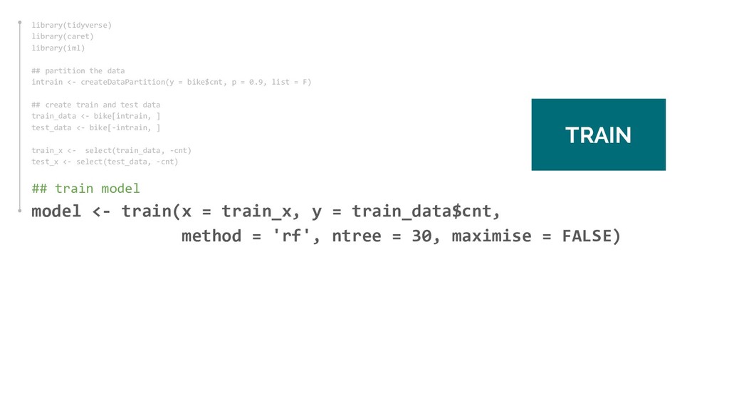
intrain <- createDataPartition(y = iris$Species,p = 0.8, list = F) ## create train and test data train_data <- iris[intrain, ] test_data <- iris[-intrain, ] ## train Random Forest model on train_data model <- train(x = train_data[, 1:4], y = train_data[, 5], method = 'rf') TRAIN
intrain <- createDataPartition(y = iris$Species, p = 0.8, list = F) ## create train and test data train_data <- iris[intrain, ] test_data <- iris[-intrain, ] ## train Random Forest model on train_data model <- train(x = train_data[, 1:4], y = train_data[, 5], method = 'rf') ## create an explainer object using train_data explainer <- lime(train_data, model) EXPLAIN
intrain <- createDataPartition(y = iris$Species, p = 0.8, list = F) ## create train and test data train_data <- iris[intrain, ] test_data <- iris[-intrain, ] ## train Random Forest model on train_data model <- train(x = train_data[, 1:4], y = train_data[, 5], method = 'rf') ## create an explainer object using train_data explainer <- lime(train_data, model) ## explain new observations in test data explanation <- explain(test_data[, 1], explainer, n_labels = 1, n_features = 4) EXPLAIN
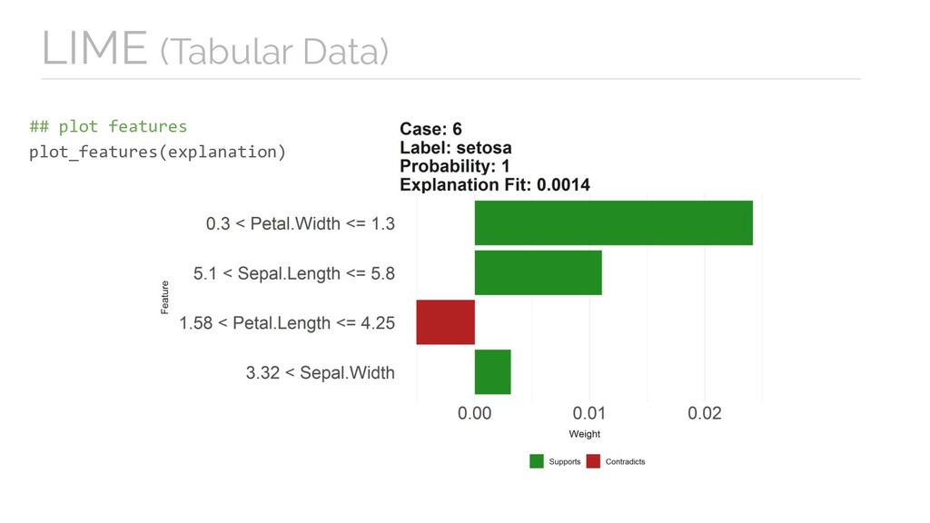
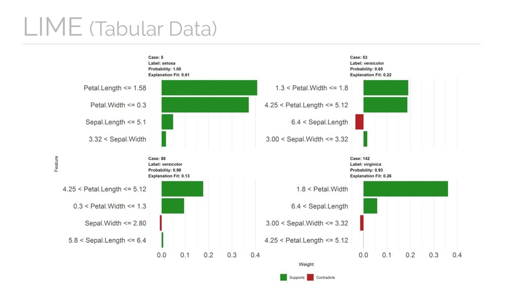
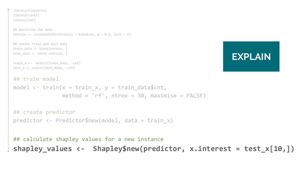
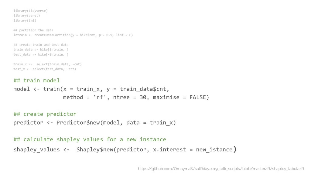
intrain <- createDataPartition(y = iris$Species, p = 0.8, list = F) ## create train and test data train_data <- iris[intrain, ] test_data <- iris[-intrain, ] ## train Random Forest model on train_data model <- train(x = train_data[, 1:4], y = train_data[, 5], method = 'rf') ## create an explainer object using train_data explainer <- lime(train_data, model) ## explain new observations in test data explanation <- explain(test_data[, 1:4], explainer, n_labels = 1, n_features = 4) https:/ /github.com/OmaymaS/satRday2019_talk_scripts/blob/master/R/lime_tabular.R
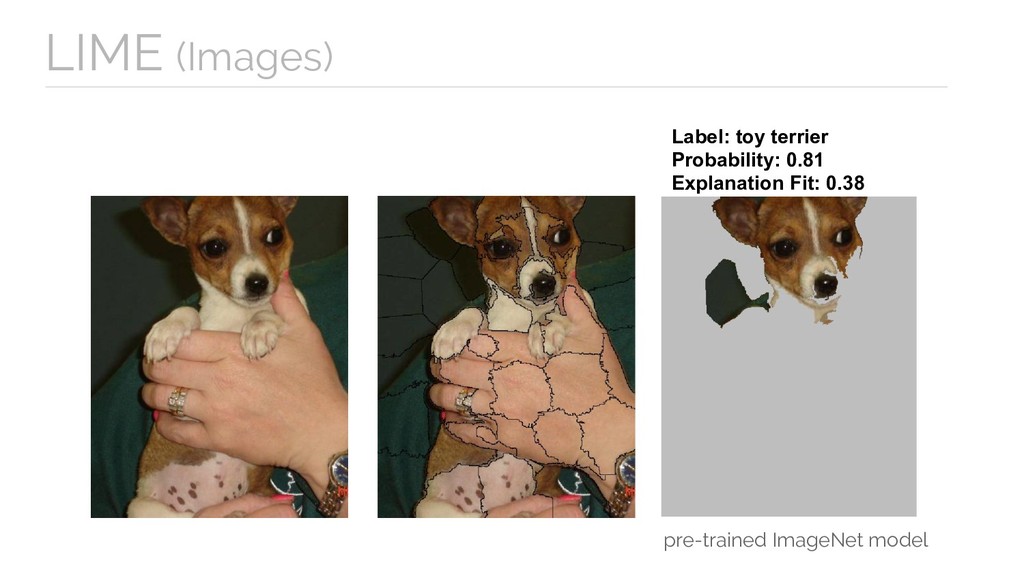
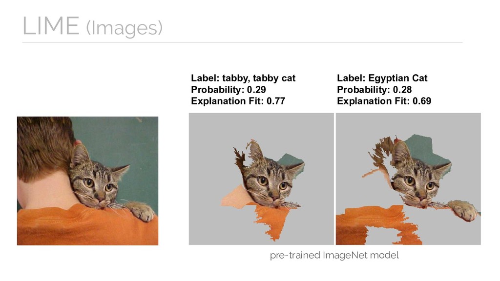
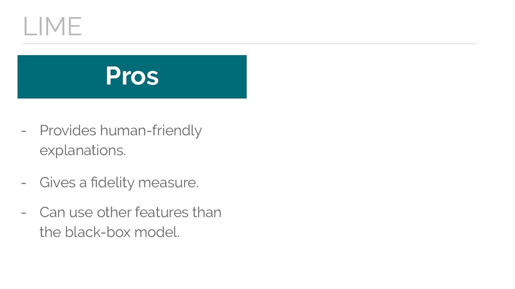
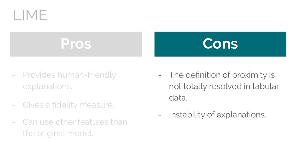
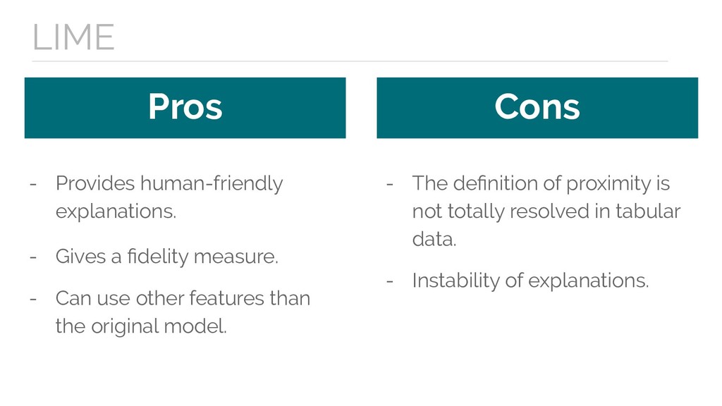
fidelity measure. - Can use other features than the original model. - The definition of proximity is not totally resolved in tabular data. - Instability of explanations.
- Can use other features than the original model. Cons - Instability of explanations. LIME - The definition of proximity is not totally resolved in tabular data.
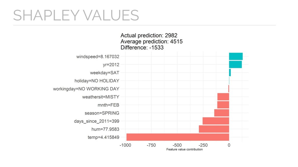
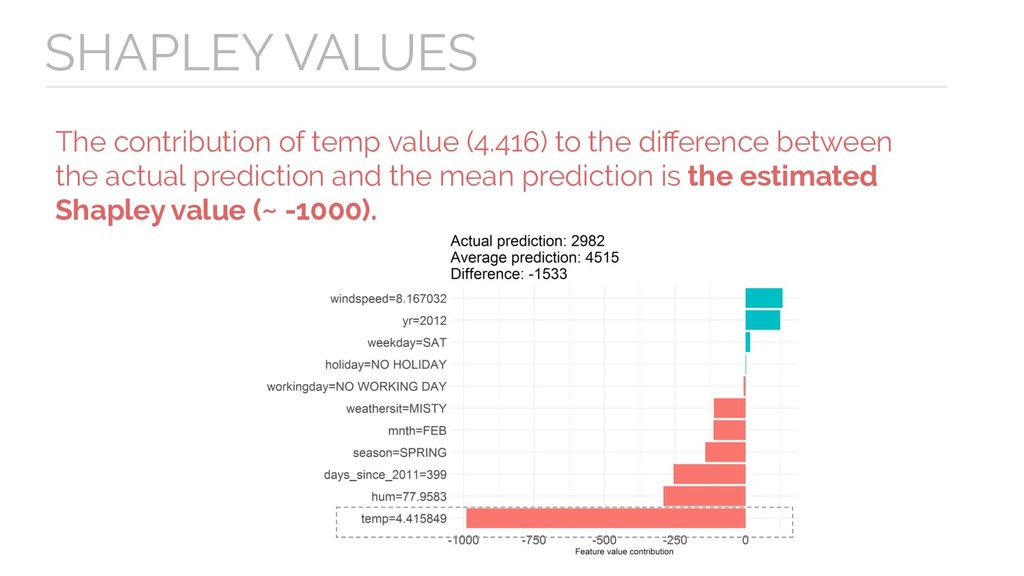
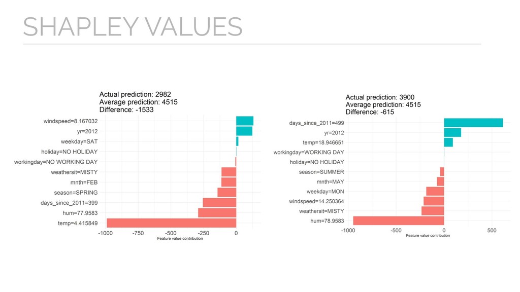
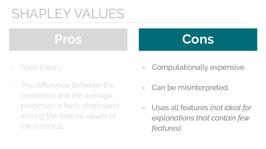
prediction and the average prediction is fairly distributed among the feature values of the instance. - Computationally expensive. - Can be misinterpreted. SHAPLEY VALUES - Uses all features (not ideal for explanations that contain few features).
prediction and the average prediction is fairly distributed among the feature values of the instance. - Computationally expensive. - Can be misinterpreted. SHAPLEY VALUES - Uses all features (not ideal for explanations that contain few features).
![AI-POWERED [----] ML-ENABLED [----] MORE AND MORE](https://files.speakerdeck.com/presentations/9ccb0fb302424f63a208f0f5ba98ba30/slide_8.jpg)
![“ ” [In Idaho], the state declined to disclose the](https://files.speakerdeck.com/presentations/9ccb0fb302424f63a208f0f5ba98ba30/slide_12.jpg)