Upgrade to Pro — share decks privately, control downloads, hide ads and more …

PWLSF#9 => Leif Walsh on Level Ancestor Simplified

PWLSF#9 => Leif Walsh on Level Ancestor Simplified

Leif Walsh , engineer at Tokutek (and from PWL NYC), comes to visit us! Leif will present the Level Ancestor Simplified paper by Bender and Farach-Colton.

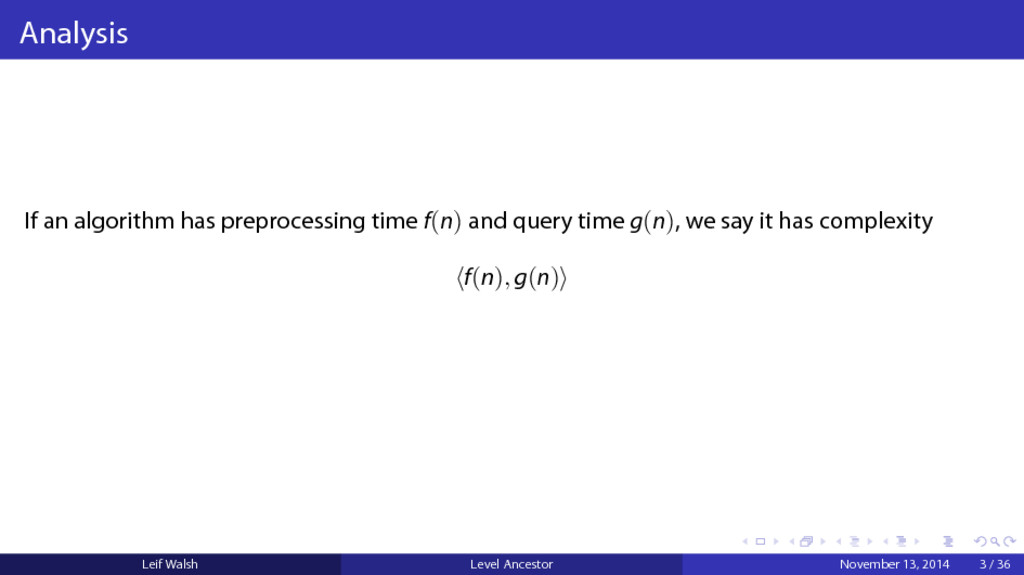
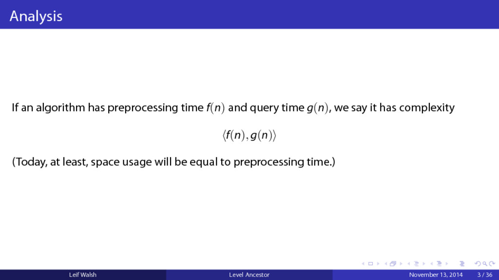
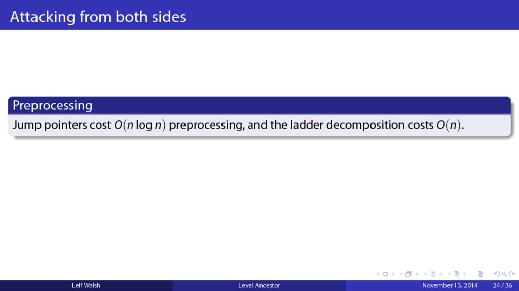
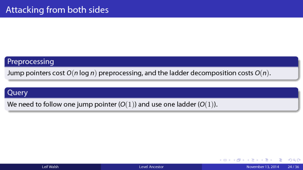
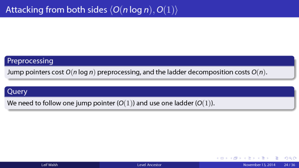
Leif tells us: " My favorite problems are always those with the highest ratio of difficulty in solving to difficulty in stating. The lowest common ancestor problem exemplifies this. It was first stated in 1973, and can be described to anyone in two sentences, or with one sentence and a picture. But it took 11 years before an optimal solution was discovered, and another 16 before an understandable and implementable solution with the same bounds was presented, in this paper, The LCA Problem Revisited. This problem is furthermore satisfying because its bounds are so tight: pre-processing takes as long as just reading the input, and queries are constant time.

The LCA Problem Revisited is a wonderfully curated journey through a deceptively simple problem that comes together in the end in a beautiful way, and it uses techniques that are powerful in plenty of other places. Plus, it solves another bonus problem along the way!"
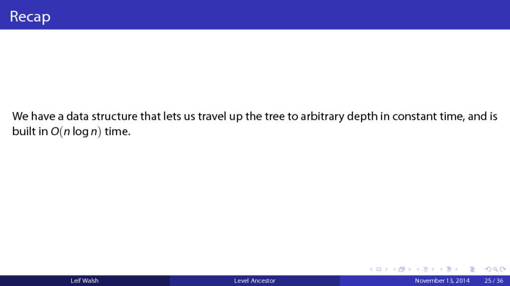
Papers_We_Love

November 13, 2014
Tweet

More Decks by Papers_We_Love

Other Decks in Technology

Transcript

  1. . . . . . . . . . .

    . . . . . . . . . . . . . . . . . . . . . . . . . . . . . . The Level Ancestor Problem simplified Leif Walsh [email protected] @leifwalsh November 13, 2014 Leif Walsh Level Ancestor November 13, 2014 1 / 36
  2. . . . . . . . . . .

    . . . . . . . . . . . . . . . . . . . . . . . . . . . . . . The Level Ancestor Problem Preprocess a rooted tree T to answer level ancestor queries: Leif Walsh Level Ancestor November 13, 2014 2 / 36
  3. . . . . . . . . . .

    . . . . . . . . . . . . . . . . . . . . . . . . . . . . . . The Level Ancestor Problem Preprocess a rooted tree T to answer level ancestor queries: T Figure: A rooted tree Definition (Depth) The depth of a node ν in a rooted tree T is the number of edges along the shortest path from the root to ν. The root has depth 0. Leif Walsh Level Ancestor November 13, 2014 2 / 36
  4. . . . . . . . . . .

    . . . . . . . . . . . . . . . . . . . . . . . . . . . . . . The Level Ancestor Problem Preprocess a rooted tree T to answer level ancestor queries: T Figure: A rooted tree Definition (Depth) The depth of a node ν in a rooted tree T is the number of edges along the shortest path from the root to ν. The root has depth 0. Definition (Level Ancestor Problem) LAT(ν, d) - return the ancestor of ν in T of depth d. LAT(ν, Depth(ν)) = ν, LAT(·, 0) = Root(T) Leif Walsh Level Ancestor November 13, 2014 2 / 36
  5. . . . . . . . . . .

    . . . . . . . . . . . . . . . . . . . . . . . . . . . . . . Analysis If an algorithm has preprocessing time f(n) and query time g(n), we say it has complexity ⟨f(n), g(n)⟩ Leif Walsh Level Ancestor November 13, 2014 3 / 36
  6. . . . . . . . . . .

    . . . . . . . . . . . . . . . . . . . . . . . . . . . . . . Analysis If an algorithm has preprocessing time f(n) and query time g(n), we say it has complexity ⟨f(n), g(n)⟩ (Today, at least, space usage will be equal to preprocessing time.) Leif Walsh Level Ancestor November 13, 2014 3 / 36
  7. . . . . . . . . . .

    . . . . . . . . . . . . . . . . . . . . . . . . . . . . . . A naïve solution Do nothing for preprocessing, walk up the tree for each query. Leif Walsh Level Ancestor November 13, 2014 4 / 36
  8. . . . . . . . . . .

    . . . . . . . . . . . . . . . . . . . . . . . . . . . . . . A naïve solution Do nothing for preprocessing, walk up the tree for each query. ⟨O(1), O(n)⟩ Leif Walsh Level Ancestor November 13, 2014 4 / 36
  9. . . . . . . . . . .

    . . . . . . . . . . . . . . . . . . . . . . . . . . . . . . The Plan We’ll proceed by presenting three simple algorithms with different characteristics: Table Algorithm Jump-Pointers Algorithm Ladder Algorithm Leif Walsh Level Ancestor November 13, 2014 5 / 36
  10. . . . . . . . . . .

    . . . . . . . . . . . . . . . . . . . . . . . . . . . . . . The Plan We’ll proceed by presenting three simple algorithms with different characteristics: Table Algorithm ⟨ O(n2), O(1) ⟩ Jump-Pointers Algorithm Ladder Algorithm Leif Walsh Level Ancestor November 13, 2014 5 / 36
  11. . . . . . . . . . .

    . . . . . . . . . . . . . . . . . . . . . . . . . . . . . . The Plan We’ll proceed by presenting three simple algorithms with different characteristics: Table Algorithm ⟨ O(n2), O(1) ⟩ Jump-Pointers Algorithm ⟨O(n log n), O(log n)⟩ Ladder Algorithm Leif Walsh Level Ancestor November 13, 2014 5 / 36
  12. . . . . . . . . . .

    . . . . . . . . . . . . . . . . . . . . . . . . . . . . . . The Plan We’ll proceed by presenting three simple algorithms with different characteristics: Table Algorithm ⟨ O(n2), O(1) ⟩ Jump-Pointers Algorithm ⟨O(n log n), O(log n)⟩ Ladder Algorithm ⟨O(n), O(log n)⟩ Leif Walsh Level Ancestor November 13, 2014 5 / 36
  13. . . . . . . . . . .

    . . . . . . . . . . . . . . . . . . . . . . . . . . . . . . The Plan We’ll proceed by presenting three simple algorithms with different characteristics: Table Algorithm ⟨ O(n2), O(1) ⟩ Jump-Pointers Algorithm ⟨O(n log n), O(log n)⟩ Ladder Algorithm ⟨O(n), O(log n)⟩ At the end, we’ll combine the last two to get a better solution. Leif Walsh Level Ancestor November 13, 2014 5 / 36
  14. . . . . . . . . . .

    . . . . . . . . . . . . . . . . . . . . . . . . . . . . . . The Plan We’ll proceed by presenting three simple algorithms with different characteristics: Table Algorithm ⟨ O(n2), O(1) ⟩ Jump-Pointers Algorithm ⟨O(n log n), O(log n)⟩ Ladder Algorithm ⟨O(n), O(log n)⟩ At the end, we’ll combine the last two to get a better solution. ⟨O(n log n), O(1)⟩ Leif Walsh Level Ancestor November 13, 2014 5 / 36
  15. . . . . . . . . . .

    . . . . . . . . . . . . . . . . . . . . . . . . . . . . . . Table Algorithm Preprocessing Precompute the answers to all possible queries LAT(ν, i) and store them in a lookup table. Leif Walsh Level Ancestor November 13, 2014 6 / 36
  16. . . . . . . . . . .

    . . . . . . . . . . . . . . . . . . . . . . . . . . . . . . Table Algorithm Preprocessing Precompute the answers to all possible queries LAT(ν, i) and store them in a lookup table. Query Look up the answer in the lookup table. Leif Walsh Level Ancestor November 13, 2014 6 / 36
  17. . . . . . . . . . .

    . . . . . . . . . . . . . . . . . . . . . . . . . . . . . . Table Algorithm Preprocessing There are n nodes in the tree, and each node ν can be queried for up to Depth(ν) different depths. Leif Walsh Level Ancestor November 13, 2014 7 / 36
  18. . . . . . . . . . .

    . . . . . . . . . . . . . . . . . . . . . . . . . . . . . . Table Algorithm Preprocessing There are n nodes in the tree, and each node ν can be queried for up to Depth(ν) different depths. Worst case: O(n2) (a stick) T Figure: A stick Leif Walsh Level Ancestor November 13, 2014 7 / 36
  19. . . . . . . . . . .

    . . . . . . . . . . . . . . . . . . . . . . . . . . . . . . Table Algorithm Preprocessing There are n nodes in the tree, and each node ν can be queried for up to Depth(ν) different depths. Worst case: O(n2) (a stick) Dynamic programming allows us to compute the whole table in O(n2). T Figure: A stick Leif Walsh Level Ancestor November 13, 2014 7 / 36
  20. . . . . . . . . . .

    . . . . . . . . . . . . . . . . . . . . . . . . . . . . . . Table Algorithm Preprocessing There are n nodes in the tree, and each node ν can be queried for up to Depth(ν) different depths. Worst case: O(n2) (a stick) Dynamic programming allows us to compute the whole table in O(n2). Query This is just array access, so O(1). T Figure: A stick Leif Walsh Level Ancestor November 13, 2014 7 / 36
  21. . . . . . . . . . .

    . . . . . . . . . . . . . . . . . . . . . . . . . . . . . . Table Algorithm ⟨ O(n2), O(1) ⟩ Preprocessing There are n nodes in the tree, and each node ν can be queried for up to Depth(ν) different depths. Worst case: O(n2) (a stick) Dynamic programming allows us to compute the whole table in O(n2). Query This is just array access, so O(1). T Figure: A stick Leif Walsh Level Ancestor November 13, 2014 7 / 36
  22. . . . . . . . . . .

    . . . . . . . . . . . . . . . . . . . . . . . . . . . . . . Jump-Pointers Algorithm Intuition: We don’t need to store every possible query from each node. We can associate less than O(n) information with each node, and still answer queries quickly. Leif Walsh Level Ancestor November 13, 2014 8 / 36
  23. . . . . . . . . . .

    . . . . . . . . . . . . . . . . . . . . . . . . . . . . . . Jump-Pointers Algorithm Intuition: We don’t need to store every possible query from each node. We can associate less than O(n) information with each node, and still answer queries quickly. To a node ν, we associate O(log n) “Jump Pointers” that let us jump up the tree from ν by powers of 2. Leif Walsh Level Ancestor November 13, 2014 8 / 36
  24. . . . . . . . . . .

    . . . . . . . . . . . . . . . . . . . . . . . . . . . . . . Jump-Pointers Algorithm T Figure: Jump pointers Leif Walsh Level Ancestor November 13, 2014 9 / 36
  25. . . . . . . . . . .

    . . . . . . . . . . . . . . . . . . . . . . . . . . . . . . Jump-Pointers Algorithm Preprocessing Compute a table Jump where Jump[ν, i] is LAT(ν, Depth(ν) − 2i), the 2i jump from ν. Leif Walsh Level Ancestor November 13, 2014 10 / 36
  26. . . . . . . . . . .

    . . . . . . . . . . . . . . . . . . . . . . . . . . . . . . Jump-Pointers Algorithm Preprocessing Compute a table Jump where Jump[ν, i] is LAT(ν, Depth(ν) − 2i), the 2i jump from ν. Query To answer a query LAT(ν, d), follow the jump pointer of maximal distance that won’t take us past depth d. Leif Walsh Level Ancestor November 13, 2014 10 / 36
  27. . . . . . . . . . .

    . . . . . . . . . . . . . . . . . . . . . . . . . . . . . . Jump-Pointers Algorithm Preprocessing Compute a table Jump where Jump[ν, i] is LAT(ν, Depth(ν) − 2i), the 2i jump from ν. Query To answer a query LAT(ν, d), follow the jump pointer of maximal distance that won’t take us past depth d. Let δ = Depth(ν) − d, Leif Walsh Level Ancestor November 13, 2014 10 / 36
  28. . . . . . . . . . .

    . . . . . . . . . . . . . . . . . . . . . . . . . . . . . . Jump-Pointers Algorithm Preprocessing Compute a table Jump where Jump[ν, i] is LAT(ν, Depth(ν) − 2i), the 2i jump from ν. Query To answer a query LAT(ν, d), follow the jump pointer of maximal distance that won’t take us past depth d. Let δ = Depth(ν) − d, then follow the jump pointer up to ν′ = Jump[ν, ⌊log δ⌋]. Leif Walsh Level Ancestor November 13, 2014 10 / 36
  29. . . . . . . . . . .

    . . . . . . . . . . . . . . . . . . . . . . . . . . . . . . Jump-Pointers Algorithm Preprocessing Compute a table Jump where Jump[ν, i] is LAT(ν, Depth(ν) − 2i), the 2i jump from ν. Query To answer a query LAT(ν, d), follow the jump pointer of maximal distance that won’t take us past depth d. Let δ = Depth(ν) − d, then follow the jump pointer up to ν′ = Jump[ν, ⌊log δ⌋]. Recursively solve LAT(ν′, d). Leif Walsh Level Ancestor November 13, 2014 10 / 36
  30. . . . . . . . . . .

    . . . . . . . . . . . . . . . . . . . . . . . . . . . . . . Jump-Pointers Algorithm x T Figure: LAT(x, 2) Leif Walsh Level Ancestor November 13, 2014 11 / 36
  31. . . . . . . . . . .

    . . . . . . . . . . . . . . . . . . . . . . . . . . . . . . Jump-Pointers Algorithm y x T Figure: LAT(x, 2) = y Leif Walsh Level Ancestor November 13, 2014 12 / 36
  32. . . . . . . . . . .

    . . . . . . . . . . . . . . . . . . . . . . . . . . . . . . Jump-Pointers Algorithm Preprocessing There are n nodes, and O(log n) jump pointers per node, so O(n log n) total pointers to compute. Dynamic programming works. Leif Walsh Level Ancestor November 13, 2014 13 / 36
  33. . . . . . . . . . .

    . . . . . . . . . . . . . . . . . . . . . . . . . . . . . . Jump-Pointers Algorithm Preprocessing There are n nodes, and O(log n) jump pointers per node, so O(n log n) total pointers to compute. Dynamic programming works. Query Each jump pointer we follow reduces δ by at least half, so we’ll reach the target in O(log n) jumps. Leif Walsh Level Ancestor November 13, 2014 13 / 36
  34. . . . . . . . . . .

    . . . . . . . . . . . . . . . . . . . . . . . . . . . . . . Jump-Pointers Algorithm ⟨O(n log n), O(log n)⟩ Preprocessing There are n nodes, and O(log n) jump pointers per node, so O(n log n) total pointers to compute. Dynamic programming works. Query Each jump pointer we follow reduces δ by at least half, so we’ll reach the target in O(log n) jumps. Leif Walsh Level Ancestor November 13, 2014 13 / 36
  35. . . . . . . . . . .

    . . . . . . . . . . . . . . . . . . . . . . . . . . . . . . Ladder Algorithm Consider a single path P. P Figure: A single path Leif Walsh Level Ancestor November 13, 2014 14 / 36
  36. . . . . . . . . . .

    . . . . . . . . . . . . . . . . . . . . . . . . . . . . . . Ladder Algorithm Consider a single path P. We can preprocess this (degenerate) tree by just putting it in an array A where A[i] corresponds to the depth-i node in the path. P Figure: A single path Leif Walsh Level Ancestor November 13, 2014 14 / 36
  37. . . . . . . . . . .

    . . . . . . . . . . . . . . . . . . . . . . . . . . . . . . Ladder Algorithm Consider a single path P. We can preprocess this (degenerate) tree by just putting it in an array A where A[i] corresponds to the depth-i node in the path. To answer LAP(·, d), just return A[d]. P Figure: A single path Leif Walsh Level Ancestor November 13, 2014 14 / 36
  38. . . . . . . . . . .

    . . . . . . . . . . . . . . . . . . . . . . . . . . . . . . Ladder Algorithm: Long-path Decomposition The long-path decomposition of a tree T is constructed as follows: Leif Walsh Level Ancestor November 13, 2014 15 / 36
  39. . . . . . . . . . .

    . . . . . . . . . . . . . . . . . . . . . . . . . . . . . . Ladder Algorithm: Long-path Decomposition The long-path decomposition of a tree T is constructed as follows: Find a longest root-to-leaf path in T, and remove it from the tree. Leif Walsh Level Ancestor November 13, 2014 15 / 36
  40. . . . . . . . . . .

    . . . . . . . . . . . . . . . . . . . . . . . . . . . . . . Ladder Algorithm: Long-path Decomposition The long-path decomposition of a tree T is constructed as follows: Find a longest root-to-leaf path in T, and remove it from the tree. Leif Walsh Level Ancestor November 13, 2014 15 / 36
  41. . . . . . . . . . .

    . . . . . . . . . . . . . . . . . . . . . . . . . . . . . . Ladder Algorithm: Long-path Decomposition The long-path decomposition of a tree T is constructed as follows: Find a longest root-to-leaf path in T, and remove it from the tree. Leif Walsh Level Ancestor November 13, 2014 15 / 36
  42. . . . . . . . . . .

    . . . . . . . . . . . . . . . . . . . . . . . . . . . . . . Ladder Algorithm: Long-path Decomposition The long-path decomposition of a tree T is constructed as follows: Find a longest root-to-leaf path in T, and remove it from the tree. Continue recursively until all remaining pieces are paths. Leif Walsh Level Ancestor November 13, 2014 15 / 36
  43. . . . . . . . . . .

    . . . . . . . . . . . . . . . . . . . . . . . . . . . . . . Ladder Algorithm: Long-path Decomposition The long-path decomposition of a tree T is constructed as follows: Find a longest root-to-leaf path in T, and remove it from the tree. Continue recursively until all remaining pieces are paths. Leif Walsh Level Ancestor November 13, 2014 15 / 36
  44. . . . . . . . . . .

    . . . . . . . . . . . . . . . . . . . . . . . . . . . . . . Ladder Algorithm: Long-path Decomposition The long-path decomposition of a tree T is constructed as follows: Find a longest root-to-leaf path in T, and remove it from the tree. Continue recursively until all remaining pieces are paths. Leif Walsh Level Ancestor November 13, 2014 15 / 36
  45. . . . . . . . . . .

    . . . . . . . . . . . . . . . . . . . . . . . . . . . . . . Ladder Algorithm: Long-path Decomposition The long-path decomposition of a tree T is constructed as follows: Find a longest root-to-leaf path in T, and remove it from the tree. Continue recursively until all remaining pieces are paths. The resulting forest of paths is the long-path decomposition. Leif Walsh Level Ancestor November 13, 2014 15 / 36
  46. . . . . . . . . . .

    . . . . . . . . . . . . . . . . . . . . . . . . . . . . . . Ladder Algorithm: Long-path Decomposition We can put each component of the long-path decomposition in a ⟨O(n), O(1)⟩ array as before, and this lets us find ancestors in our component in O(1). Leif Walsh Level Ancestor November 13, 2014 16 / 36
  47. . . . . . . . . . .

    . . . . . . . . . . . . . . . . . . . . . . . . . . . . . . Ladder Algorithm: Long-path Decomposition We can put each component of the long-path decomposition in a ⟨O(n), O(1)⟩ array as before, and this lets us find ancestors in our component in O(1). However, if we need to go higher, we need to step up to the next component higher and continue. Leif Walsh Level Ancestor November 13, 2014 16 / 36
  48. . . . . . . . . . .

    . . . . . . . . . . . . . . . . . . . . . . . . . . . . . . Ladder Algorithm: Long-path Decomposition We can put each component of the long-path decomposition in a ⟨O(n), O(1)⟩ array as before, and this lets us find ancestors in our component in O(1). However, if we need to go higher, we need to step up to the next component higher and continue. In the worst case, querying this structure can take O( √ n). Figure: Worst case for long path decomposition. Leif Walsh Level Ancestor November 13, 2014 16 / 36
  49. . . . . . . . . . .

    . . . . . . . . . . . . . . . . . . . . . . . . . . . . . . Ladder Algorithm: Ladder Decomposition We will augment the long-path decomposition, to essentially let us climb higher in a single array, and avoid checking O( √ n) separate arrays. Leif Walsh Level Ancestor November 13, 2014 17 / 36
  50. . . . . . . . . . .

    . . . . . . . . . . . . . . . . . . . . . . . . . . . . . . Ladder Algorithm: Ladder Decomposition We will augment the long-path decomposition, to essentially let us climb higher in a single array, and avoid checking O( √ n) separate arrays. For each component in the long-path decomposition (of height h), we previously created an array of size h to represent it. Leif Walsh Level Ancestor November 13, 2014 17 / 36
  51. . . . . . . . . . .

    . . . . . . . . . . . . . . . . . . . . . . . . . . . . . . Ladder Algorithm: Ladder Decomposition We will augment the long-path decomposition, to essentially let us climb higher in a single array, and avoid checking O( √ n) separate arrays. For each component in the long-path decomposition (of height h), we previously created an array of size h to represent it. Now, we allocate an array of size 2h, and in addition to storing the component, we also store the h ancestors directly above the component. Leif Walsh Level Ancestor November 13, 2014 17 / 36
  52. . . . . . . . . . .

    . . . . . . . . . . . . . . . . . . . . . . . . . . . . . . Ladder Algorithm: Ladder Decomposition We will augment the long-path decomposition, to essentially let us climb higher in a single array, and avoid checking O( √ n) separate arrays. For each component in the long-path decomposition (of height h), we previously created an array of size h to represent it. Now, we allocate an array of size 2h, and in addition to storing the component, we also store the h ancestors directly above the component. This doubles our storage and preprocessing work, but gives us some nice properties. We’ll call these augmented arrays ladders. Leif Walsh Level Ancestor November 13, 2014 17 / 36
  53. . . . . . . . . . .

    . . . . . . . . . . . . . . . . . . . . . . . . . . . . . . Ladder Algorithm: Ladder Decomposition We will augment the long-path decomposition, to essentially let us climb higher in a single array, and avoid checking O( √ n) separate arrays. For each component in the long-path decomposition (of height h), we previously created an array of size h to represent it. Now, we allocate an array of size 2h, and in addition to storing the component, we also store the h ancestors directly above the component. This doubles our storage and preprocessing work, but gives us some nice properties. We’ll call these augmented arrays ladders. Leif Walsh Level Ancestor November 13, 2014 17 / 36
  54. . . . . . . . . . .

    . . . . . . . . . . . . . . . . . . . . . . . . . . . . . . Ladder Algorithm: Ladder Decomposition We will augment the long-path decomposition, to essentially let us climb higher in a single array, and avoid checking O( √ n) separate arrays. For each component in the long-path decomposition (of height h), we previously created an array of size h to represent it. Now, we allocate an array of size 2h, and in addition to storing the component, we also store the h ancestors directly above the component. This doubles our storage and preprocessing work, but gives us some nice properties. We’ll call these augmented arrays ladders. Leif Walsh Level Ancestor November 13, 2014 17 / 36
  55. . . . . . . . . . .

    . . . . . . . . . . . . . . . . . . . . . . . . . . . . . . Ladder Algorithm: Ladder Decomposition We will augment the long-path decomposition, to essentially let us climb higher in a single array, and avoid checking O( √ n) separate arrays. For each component in the long-path decomposition (of height h), we previously created an array of size h to represent it. Now, we allocate an array of size 2h, and in addition to storing the component, we also store the h ancestors directly above the component. This doubles our storage and preprocessing work, but gives us some nice properties. We’ll call these augmented arrays ladders. Leif Walsh Level Ancestor November 13, 2014 17 / 36
  56. . . . . . . . . . .

    . . . . . . . . . . . . . . . . . . . . . . . . . . . . . . Ladder Algorithm: Ladder Decomposition We will augment the long-path decomposition, to essentially let us climb higher in a single array, and avoid checking O( √ n) separate arrays. For each component in the long-path decomposition (of height h), we previously created an array of size h to represent it. Now, we allocate an array of size 2h, and in addition to storing the component, we also store the h ancestors directly above the component. This doubles our storage and preprocessing work, but gives us some nice properties. We’ll call these augmented arrays ladders. Leif Walsh Level Ancestor November 13, 2014 17 / 36
  57. . . . . . . . . . .

    . . . . . . . . . . . . . . . . . . . . . . . . . . . . . . Ladder Algorithm: Ladder Decomposition We will augment the long-path decomposition, to essentially let us climb higher in a single array, and avoid checking O( √ n) separate arrays. For each component in the long-path decomposition (of height h), we previously created an array of size h to represent it. Now, we allocate an array of size 2h, and in addition to storing the component, we also store the h ancestors directly above the component. This doubles our storage and preprocessing work, but gives us some nice properties. We’ll call these augmented arrays ladders. Leif Walsh Level Ancestor November 13, 2014 17 / 36
  58. . . . . . . . . . .

    . . . . . . . . . . . . . . . . . . . . . . . . . . . . . . Ladder Algorithm: Ladder Decomposition We will augment the long-path decomposition, to essentially let us climb higher in a single array, and avoid checking O( √ n) separate arrays. For each component in the long-path decomposition (of height h), we previously created an array of size h to represent it. Now, we allocate an array of size 2h, and in addition to storing the component, we also store the h ancestors directly above the component. This doubles our storage and preprocessing work, but gives us some nice properties. We’ll call these augmented arrays ladders. Leif Walsh Level Ancestor November 13, 2014 17 / 36
  59. . . . . . . . . . .

    . . . . . . . . . . . . . . . . . . . . . . . . . . . . . . Ladder Algorithm: Ladder Decomposition We will augment the long-path decomposition, to essentially let us climb higher in a single array, and avoid checking O( √ n) separate arrays. For each component in the long-path decomposition (of height h), we previously created an array of size h to represent it. Now, we allocate an array of size 2h, and in addition to storing the component, we also store the h ancestors directly above the component. This doubles our storage and preprocessing work, but gives us some nice properties. We’ll call these augmented arrays ladders. Leif Walsh Level Ancestor November 13, 2014 17 / 36
  60. . . . . . . . . . .

    . . . . . . . . . . . . . . . . . . . . . . . . . . . . . . Ladder Algorithm: Ladder Decomposition Definition (Height) The height of a node ν in a tree T is the number of nodes on the longest path from ν to any descendant. Leaves have height 1. Leif Walsh Level Ancestor November 13, 2014 18 / 36
  61. . . . . . . . . . .

    . . . . . . . . . . . . . . . . . . . . . . . . . . . . . . Ladder Algorithm: Ladder Decomposition Definition (Height) The height of a node ν in a tree T is the number of nodes on the longest path from ν to any descendant. Leaves have height 1. Property Consider a node ν of height h. The top of ν’s ladder is at least distance h above ν. That is, we can jump up ν’s ladder by at least h in O(1) time. Leif Walsh Level Ancestor November 13, 2014 18 / 36
  62. . . . . . . . . . .

    . . . . . . . . . . . . . . . . . . . . . . . . . . . . . . Ladder Algorithm: Ladder Decomposition Definition (Height) The height of a node ν in a tree T is the number of nodes on the longest path from ν to any descendant. Leaves have height 1. Property Consider a node ν of height h. The top of ν’s ladder is at least distance h above ν. That is, we can jump up ν’s ladder by at least h in O(1) time. Corollary If a node ν has height h, then ν’s ladder either includes a node of height 2h, or it includes the entire path from the root to ν, and therefore all of ν’s ancestors. Leif Walsh Level Ancestor November 13, 2014 18 / 36
  63. . . . . . . . . . .

    . . . . . . . . . . . . . . . . . . . . . . . . . . . . . . Ladder Algorithm Preprocessing Construct the long-path decomposition of T, by precomputing heights in one DFS pass, and in a second pass, greedily following the maximal-height child at each node. Extend each component to a ladder by following parent pointers. Leif Walsh Level Ancestor November 13, 2014 19 / 36
  64. . . . . . . . . . .

    . . . . . . . . . . . . . . . . . . . . . . . . . . . . . . Ladder Algorithm Preprocessing Construct the long-path decomposition of T, by precomputing heights in one DFS pass, and in a second pass, greedily following the maximal-height child at each node. Extend each component to a ladder by following parent pointers. Query To answer LAT(ν, d), consider ν’s ladder. If it is tall enough to contain the depth-d ancestor, we are done. Otherwise, jump to the node at the top of ν’s ladder, and try again from that node’s ladder. Leif Walsh Level Ancestor November 13, 2014 19 / 36
  65. . . . . . . . . . .

    . . . . . . . . . . . . . . . . . . . . . . . . . . . . . . Ladder Algorithm Preprocessing The long-path decomposition just takes a couple O(n) traversals of the tree. Extending the components into ladders costs another O(n), because each ancestor we touch to augment a ladder can be charged to a node in the component. Leif Walsh Level Ancestor November 13, 2014 20 / 36
  66. . . . . . . . . . .

    . . . . . . . . . . . . . . . . . . . . . . . . . . . . . . Ladder Algorithm Preprocessing The long-path decomposition just takes a couple O(n) traversals of the tree. Extending the components into ladders costs another O(n), because each ancestor we touch to augment a ladder can be charged to a node in the component. Query Jumping up to a higher ladder costs O(1), it’s just array access. Each time we step up from a ladder of height h, we find ourselves in a ladder of height ≥ 2h. Since all ladders are of height at least 1, after i ladders we reach a node of height at least 2i. The ancestor we want has height at most n, so we reach it after visiting O(log n) ladders. Leif Walsh Level Ancestor November 13, 2014 20 / 36
  67. . . . . . . . . . .

    . . . . . . . . . . . . . . . . . . . . . . . . . . . . . . Ladder Algorithm ⟨O(n), O(log n)⟩ Preprocessing The long-path decomposition just takes a couple O(n) traversals of the tree. Extending the components into ladders costs another O(n), because each ancestor we touch to augment a ladder can be charged to a node in the component. Query Jumping up to a higher ladder costs O(1), it’s just array access. Each time we step up from a ladder of height h, we find ourselves in a ladder of height ≥ 2h. Since all ladders are of height at least 1, after i ladders we reach a node of height at least 2i. The ancestor we want has height at most n, so we reach it after visiting O(log n) ladders. Leif Walsh Level Ancestor November 13, 2014 20 / 36
  68. . . . . . . . . . .

    . . . . . . . . . . . . . . . . . . . . . . . . . . . . . . Attacking from both sides Leif Walsh Level Ancestor November 13, 2014 21 / 36
  69. . . . . . . . . . .

    . . . . . . . . . . . . . . . . . . . . . . . . . . . . . . Attacking from both sides Leif Walsh Level Ancestor November 13, 2014 21 / 36
  70. . . . . . . . . . .

    . . . . . . . . . . . . . . . . . . . . . . . . . . . . . . Attacking from both sides Why do these algorithms (Jump Pointers and Ladders) work? Leif Walsh Level Ancestor November 13, 2014 22 / 36
  71. . . . . . . . . . .

    . . . . . . . . . . . . . . . . . . . . . . . . . . . . . . Attacking from both sides Why do these algorithms (Jump Pointers and Ladders) work? Jump pointers allow us to cover a lot of ground quickly: at least half the distance to our destination in the first step. Leif Walsh Level Ancestor November 13, 2014 22 / 36
  72. . . . . . . . . . .

    . . . . . . . . . . . . . . . . . . . . . . . . . . . . . . Attacking from both sides Why do these algorithms (Jump Pointers and Ladders) work? Jump pointers allow us to cover a lot of ground quickly: at least half the distance to our destination in the first step. Ladders start out slowly, but once you’re halfway to the destination, you get there in one more jump. Leif Walsh Level Ancestor November 13, 2014 22 / 36
  73. . . . . . . . . . .

    . . . . . . . . . . . . . . . . . . . . . . . . . . . . . . Attacking from both sides Preprocessing Construct both the jump pointers and the ladder decomposition of T. Leif Walsh Level Ancestor November 13, 2014 23 / 36
  74. . . . . . . . . . .

    . . . . . . . . . . . . . . . . . . . . . . . . . . . . . . Attacking from both sides Preprocessing Construct both the jump pointers and the ladder decomposition of T. Query Consider LAT(ν, d). We need to travel up δ = Depth(ν) − d. Leif Walsh Level Ancestor November 13, 2014 23 / 36
  75. . . . . . . . . . .

    . . . . . . . . . . . . . . . . . . . . . . . . . . . . . . Attacking from both sides Preprocessing Construct both the jump pointers and the ladder decomposition of T. Query Consider LAT(ν, d). We need to travel up δ = Depth(ν) − d. One step of the jump pointer algorithm takes us to a node ν′ at least δ/2 higher than ν. Leif Walsh Level Ancestor November 13, 2014 23 / 36
  76. . . . . . . . . . .

    . . . . . . . . . . . . . . . . . . . . . . . . . . . . . . Attacking from both sides Preprocessing Construct both the jump pointers and the ladder decomposition of T. Query Consider LAT(ν, d). We need to travel up δ = Depth(ν) − d. One step of the jump pointer algorithm takes us to a node ν′ at least δ/2 higher than ν. This node ν′ has height h′ ≥ δ/2. The ladder for ν′ must extend higher by at least another h′, which is enough to take us the rest of the way. Leif Walsh Level Ancestor November 13, 2014 23 / 36
  77. . . . . . . . . . .

    . . . . . . . . . . . . . . . . . . . . . . . . . . . . . . Attacking from both sides Preprocessing Jump pointers cost O(n log n) preprocessing, and the ladder decomposition costs O(n). Leif Walsh Level Ancestor November 13, 2014 24 / 36
  78. . . . . . . . . . .

    . . . . . . . . . . . . . . . . . . . . . . . . . . . . . . Attacking from both sides Preprocessing Jump pointers cost O(n log n) preprocessing, and the ladder decomposition costs O(n). Query We need to follow one jump pointer (O(1)) and use one ladder (O(1)). Leif Walsh Level Ancestor November 13, 2014 24 / 36
  79. . . . . . . . . . .

    . . . . . . . . . . . . . . . . . . . . . . . . . . . . . . Attacking from both sides ⟨O(n log n), O(1)⟩ Preprocessing Jump pointers cost O(n log n) preprocessing, and the ladder decomposition costs O(n). Query We need to follow one jump pointer (O(1)) and use one ladder (O(1)). Leif Walsh Level Ancestor November 13, 2014 24 / 36
  80. . . . . . . . . . .

    . . . . . . . . . . . . . . . . . . . . . . . . . . . . . . Recap We have a data structure that lets us travel up the tree to arbitrary depth in constant time, and is built in O(n log n) time. Leif Walsh Level Ancestor November 13, 2014 25 / 36
  81. . . . . . . . . . .

    . . . . . . . . . . . . . . . . . . . . . . . . . . . . . . Recap We have a data structure that lets us travel up the tree to arbitrary depth in constant time, and is built in O(n log n) time. Now let’s build it in linear time. Leif Walsh Level Ancestor November 13, 2014 25 / 36
  82. . . . . . . . . . .

    . . . . . . . . . . . . . . . . . . . . . . . . . . . . . . Mathematicians HATE me for this one weird trick... Leif Walsh Level Ancestor November 13, 2014 26 / 36
  83. . . . . . . . . . .

    . . . . . . . . . . . . . . . . . . . . . . . . . . . . . . One weird math trick... Consider a problem of size n. Leif Walsh Level Ancestor November 13, 2014 27 / 36
  84. . . . . . . . . . .

    . . . . . . . . . . . . . . . . . . . . . . . . . . . . . . One weird math trick... Consider a problem of size n. We will divide this into O(n/ log n) subproblems each of size O(log n), and one superproblem of size O(n/ log n). Leif Walsh Level Ancestor November 13, 2014 27 / 36
  85. . . . . . . . . . .

    . . . . . . . . . . . . . . . . . . . . . . . . . . . . . . One weird math trick... Consider a problem of size n. We will divide this into O(n/ log n) subproblems each of size O(log n), and one superproblem of size O(n/ log n). We’ll use an O(n log n) algorithm to solve the superproblem, and then we just have small problems left to solve, which we’ll also solve quickly. Leif Walsh Level Ancestor November 13, 2014 27 / 36
  86. . . . . . . . . . .

    . . . . . . . . . . . . . . . . . . . . . . . . . . . . . . One weird math trick... Let m = O(n/ log n) be the size of the superproblem. The preprocessing complexity for the superproblem is: Leif Walsh Level Ancestor November 13, 2014 28 / 36
  87. . . . . . . . . . .

    . . . . . . . . . . . . . . . . . . . . . . . . . . . . . . One weird math trick... Let m = O(n/ log n) be the size of the superproblem. The preprocessing complexity for the superproblem is: O(m log m) = O ( n log n log ( n log n )) Leif Walsh Level Ancestor November 13, 2014 28 / 36
  88. . . . . . . . . . .

    . . . . . . . . . . . . . . . . . . . . . . . . . . . . . . One weird math trick... Let m = O(n/ log n) be the size of the superproblem. The preprocessing complexity for the superproblem is: O(m log m) = O ( n log n log ( n log n )) = O ( n log n (log n − log log n) ) Leif Walsh Level Ancestor November 13, 2014 28 / 36
  89. . . . . . . . . . .

    . . . . . . . . . . . . . . . . . . . . . . . . . . . . . . One weird math trick... Let m = O(n/ log n) be the size of the superproblem. The preprocessing complexity for the superproblem is: O(m log m) = O ( n log n log ( n log n )) = O ( n log n (log n − log log n) ) = O ( n log n log n ) Leif Walsh Level Ancestor November 13, 2014 28 / 36
  90. . . . . . . . . . .

    . . . . . . . . . . . . . . . . . . . . . . . . . . . . . . One weird math trick... Let m = O(n/ log n) be the size of the superproblem. The preprocessing complexity for the superproblem is: O(m log m) = O ( n log n log ( n log n )) = O ( n log n (log n − log log n) ) = O ( n log n log n ) Leif Walsh Level Ancestor November 13, 2014 28 / 36
  91. . . . . . . . . . .

    . . . . . . . . . . . . . . . . . . . . . . . . . . . . . . One weird math trick... Let m = O(n/ log n) be the size of the superproblem. The preprocessing complexity for the superproblem is: O(m log m) = O ( n log n log ( n log n )) = O ( n log n (log n − log log n) ) = O ( n log n log n ) = O (n) Leif Walsh Level Ancestor November 13, 2014 28 / 36
  92. . . . . . . . . . .

    . . . . . . . . . . . . . . . . . . . . . . . . . . . . . . Macro-Micro-Tree Algorithm We choose Jump Nodes as the maximally deep nodes with at least log(n)/4 descendants Leif Walsh Level Ancestor November 13, 2014 29 / 36
  93. . . . . . . . . . .

    . . . . . . . . . . . . . . . . . . . . . . . . . . . . . . Macro-Micro-Tree Algorithm We choose Jump Nodes as the maximally deep nodes with at least log(n)/4 descendants Leif Walsh Level Ancestor November 13, 2014 29 / 36
  94. . . . . . . . . . .

    . . . . . . . . . . . . . . . . . . . . . . . . . . . . . . Macro-Micro-Tree Algorithm We choose Jump Nodes as the maximally deep nodes with at least log(n)/4 descendants This gives us many “micro trees” of size less than log(n)/4, and one “macro tree” of size O(n/ log n). The macro tree has the jump nodes as its leaves. Leif Walsh Level Ancestor November 13, 2014 29 / 36
  95. . . . . . . . . . .

    . . . . . . . . . . . . . . . . . . . . . . . . . . . . . . Macro-Micro-Tree Algorithm We choose Jump Nodes as the maximally deep nodes with at least log(n)/4 descendants This gives us many “micro trees” of size less than log(n)/4, and one “macro tree” of size O(n/ log n). The macro tree has the jump nodes as its leaves. We compute jump pointers only for these jump nodes, and for all other nodes ν in the macro tree, we assign JumpDesc(ν) to be one of its jump node descendants. Leif Walsh Level Ancestor November 13, 2014 29 / 36
  96. . . . . . . . . . .

    . . . . . . . . . . . . . . . . . . . . . . . . . . . . . . Macro-Micro-Tree Algorithm We choose Jump Nodes as the maximally deep nodes with at least log(n)/4 descendants This gives us many “micro trees” of size less than log(n)/4, and one “macro tree” of size O(n/ log n). The macro tree has the jump nodes as its leaves. We compute jump pointers only for these jump nodes, and for all other nodes ν in the macro tree, we assign JumpDesc(ν) to be one of its jump node descendants. Leif Walsh Level Ancestor November 13, 2014 29 / 36
  97. . . . . . . . . . .

    . . . . . . . . . . . . . . . . . . . . . . . . . . . . . . Macro-Micro-Tree Algorithm To solve a query LAT(ν, d) where ν is in the macro tree, we first jump down to JumpDesc(ν), then use one of its jump pointers and then one ladder to find LAT(JumpDesc(ν), d) = LAT(ν, d). Leif Walsh Level Ancestor November 13, 2014 30 / 36
  98. . . . . . . . . . .

    . . . . . . . . . . . . . . . . . . . . . . . . . . . . . . Macro-Micro-Tree Algorithm If the query is in one of the micro trees, we need a strategy to solve it. Leif Walsh Level Ancestor November 13, 2014 31 / 36
  99. . . . . . . . . . .

    . . . . . . . . . . . . . . . . . . . . . . . . . . . . . . Macro-Micro-Tree Algorithm If the query is in one of the micro trees, we need a strategy to solve it. Consider a DFS on a micro tree. We visit each edge twice, first going down, then later, going up. We can identify a tree shape with m nodes with a bit vector, representing the DFS, of length 2(m − 1). Leif Walsh Level Ancestor November 13, 2014 31 / 36
  100. . . . . . . . . . .

    . . . . . . . . . . . . . . . . . . . . . . . . . . . . . . Macro-Micro-Tree Algorithm If the query is in one of the micro trees, we need a strategy to solve it. Consider a DFS on a micro tree. We visit each edge twice, first going down, then later, going up. We can identify a tree shape with m nodes with a bit vector, representing the DFS, of length 2(m − 1). 0 Leif Walsh Level Ancestor November 13, 2014 31 / 36
  101. . . . . . . . . . .

    . . . . . . . . . . . . . . . . . . . . . . . . . . . . . . Macro-Micro-Tree Algorithm If the query is in one of the micro trees, we need a strategy to solve it. Consider a DFS on a micro tree. We visit each edge twice, first going down, then later, going up. We can identify a tree shape with m nodes with a bit vector, representing the DFS, of length 2(m − 1). 0 0 Leif Walsh Level Ancestor November 13, 2014 31 / 36
  102. . . . . . . . . . .

    . . . . . . . . . . . . . . . . . . . . . . . . . . . . . . Macro-Micro-Tree Algorithm If the query is in one of the micro trees, we need a strategy to solve it. Consider a DFS on a micro tree. We visit each edge twice, first going down, then later, going up. We can identify a tree shape with m nodes with a bit vector, representing the DFS, of length 2(m − 1). 0 0 1 Leif Walsh Level Ancestor November 13, 2014 31 / 36
  103. . . . . . . . . . .

    . . . . . . . . . . . . . . . . . . . . . . . . . . . . . . Macro-Micro-Tree Algorithm If the query is in one of the micro trees, we need a strategy to solve it. Consider a DFS on a micro tree. We visit each edge twice, first going down, then later, going up. We can identify a tree shape with m nodes with a bit vector, representing the DFS, of length 2(m − 1). 0 0 1 0 Leif Walsh Level Ancestor November 13, 2014 31 / 36
  104. . . . . . . . . . .

    . . . . . . . . . . . . . . . . . . . . . . . . . . . . . . Macro-Micro-Tree Algorithm If the query is in one of the micro trees, we need a strategy to solve it. Consider a DFS on a micro tree. We visit each edge twice, first going down, then later, going up. We can identify a tree shape with m nodes with a bit vector, representing the DFS, of length 2(m − 1). 0 0 1 0 1 Leif Walsh Level Ancestor November 13, 2014 31 / 36
  105. . . . . . . . . . .

    . . . . . . . . . . . . . . . . . . . . . . . . . . . . . . Macro-Micro-Tree Algorithm If the query is in one of the micro trees, we need a strategy to solve it. Consider a DFS on a micro tree. We visit each edge twice, first going down, then later, going up. We can identify a tree shape with m nodes with a bit vector, representing the DFS, of length 2(m − 1). 0 0 1 0 1 1 Leif Walsh Level Ancestor November 13, 2014 31 / 36
  106. . . . . . . . . . .

    . . . . . . . . . . . . . . . . . . . . . . . . . . . . . . Macro-Micro-Tree Algorithm If the query is in one of the micro trees, we need a strategy to solve it. Consider a DFS on a micro tree. We visit each edge twice, first going down, then later, going up. We can identify a tree shape with m nodes with a bit vector, representing the DFS, of length 2(m − 1). 0 0 1 0 1 1 0 Leif Walsh Level Ancestor November 13, 2014 31 / 36
  107. . . . . . . . . . .

    . . . . . . . . . . . . . . . . . . . . . . . . . . . . . . Macro-Micro-Tree Algorithm If the query is in one of the micro trees, we need a strategy to solve it. Consider a DFS on a micro tree. We visit each edge twice, first going down, then later, going up. We can identify a tree shape with m nodes with a bit vector, representing the DFS, of length 2(m − 1). 0 0 1 0 1 1 0 1 Leif Walsh Level Ancestor November 13, 2014 31 / 36
  108. . . . . . . . . . .

    . . . . . . . . . . . . . . . . . . . . . . . . . . . . . . Macro-Micro-Tree Algorithm If the query is in one of the micro trees, we need a strategy to solve it. Consider a DFS on a micro tree. We visit each edge twice, first going down, then later, going up. We can identify a tree shape with m nodes with a bit vector, representing the DFS, of length 2(m − 1). Each micro tree has less than log(n)/4 nodes, so there are few possible shapes of micro tree: 0 0 1 0 1 1 0 1 Leif Walsh Level Ancestor November 13, 2014 31 / 36
  109. . . . . . . . . . .

    . . . . . . . . . . . . . . . . . . . . . . . . . . . . . . Macro-Micro-Tree Algorithm If the query is in one of the micro trees, we need a strategy to solve it. Consider a DFS on a micro tree. We visit each edge twice, first going down, then later, going up. We can identify a tree shape with m nodes with a bit vector, representing the DFS, of length 2(m − 1). Each micro tree has less than log(n)/4 nodes, so there are few possible shapes of micro tree: 22(m−1) ≤ 2log(n)/2 = ( 2log n )1 2 = √ n 0 0 1 0 1 1 0 1 Leif Walsh Level Ancestor November 13, 2014 31 / 36
  110. . . . . . . . . . .

    . . . . . . . . . . . . . . . . . . . . . . . . . . . . . . Macro-Micro-Tree Algorithm We’ll use the simple ⟨ O(n2), O(1) ⟩ Table Algorithm to preprocess every possible micro tree shape. Leif Walsh Level Ancestor November 13, 2014 32 / 36
  111. . . . . . . . . . .

    . . . . . . . . . . . . . . . . . . . . . . . . . . . . . . Macro-Micro-Tree Algorithm We’ll use the simple ⟨ O(n2), O(1) ⟩ Table Algorithm to preprocess every possible micro tree shape. To answer a query LAT(ν, d) when ν is in a micro tree, either: Use the Table Algorithm if the target is in the micro tree. Jump to the root of the micro tree and use the macro tree algorithm from its parent. Leif Walsh Level Ancestor November 13, 2014 32 / 36
  112. . . . . . . . . . .

    . . . . . . . . . . . . . . . . . . . . . . . . . . . . . . Macro-Micro-Tree Algorithm Preprocessing As before, we can build the Ladder Algorithm’s data structure in O(n) time. Leif Walsh Level Ancestor November 13, 2014 33 / 36
  113. . . . . . . . . . .

    . . . . . . . . . . . . . . . . . . . . . . . . . . . . . . Macro-Micro-Tree Algorithm Preprocessing As before, we can build the Ladder Algorithm’s data structure in O(n) time. We can identify the jump nodes and the micro trees with DFS. We can compute jump pointers for the jump nodes, using the ladders, in O(log n) time per jump node. There are O(n/ log n) jump nodes, so computing all jump pointers takes O(n) time. Leif Walsh Level Ancestor November 13, 2014 33 / 36
  114. . . . . . . . . . .

    . . . . . . . . . . . . . . . . . . . . . . . . . . . . . . Macro-Micro-Tree Algorithm Preprocessing As before, we can build the Ladder Algorithm’s data structure in O(n) time. We can identify the jump nodes and the micro trees with DFS. We can compute jump pointers for the jump nodes, using the ladders, in O(log n) time per jump node. There are O(n/ log n) jump nodes, so computing all jump pointers takes O(n) time. Preprocessing one micro tree costs O(log2 n), so all microtrees together have complexity O( √ n log2 n) ≤ O(n). Leif Walsh Level Ancestor November 13, 2014 33 / 36
  115. . . . . . . . . . .

    . . . . . . . . . . . . . . . . . . . . . . . . . . . . . . Macro-Micro-Tree Algorithm Query If the query is in the macro tree, we jump down to a jump node, use one jump pointer, and one ladder, which are all O(1). Leif Walsh Level Ancestor November 13, 2014 34 / 36
  116. . . . . . . . . . .

    . . . . . . . . . . . . . . . . . . . . . . . . . . . . . . Macro-Micro-Tree Algorithm Query If the query is in the macro tree, we jump down to a jump node, use one jump pointer, and one ladder, which are all O(1). If the query is in the micro tree, we solve it there with the Table Algorithm in O(1) time, or use the macro tree, which is also O(1) as above. Leif Walsh Level Ancestor November 13, 2014 34 / 36
  117. . . . . . . . . . .

    . . . . . . . . . . . . . . . . . . . . . . . . . . . . . . Macro-Micro-Tree Algorithm ⟨O(n), O(1)⟩ Query If the query is in the macro tree, we jump down to a jump node, use one jump pointer, and one ladder, which are all O(1). If the query is in the micro tree, we solve it there with the Table Algorithm in O(1) time, or use the macro tree, which is also O(1) as above. Leif Walsh Level Ancestor November 13, 2014 34 / 36
  118. . . . . . . . . . .

    . . . . . . . . . . . . . . . . . . . . . . . . . . . . . . Lessons Leif Walsh Level Ancestor November 13, 2014 35 / 36
  119. . . . . . . . . . .

    . . . . . . . . . . . . . . . . . . . . . . . . . . . . . . Lessons Look for paired algorithms that complement each other by reinforcing each others’ weaknesses (Ladders and Jump Pointers). Leif Walsh Level Ancestor November 13, 2014 35 / 36
  120. . . . . . . . . . .

    . . . . . . . . . . . . . . . . . . . . . . . . . . . . . . Lessons Look for paired algorithms that complement each other by reinforcing each others’ weaknesses (Ladders and Jump Pointers). Turn an O(n log n) algorithm into an O(n) algorithm: Leif Walsh Level Ancestor November 13, 2014 35 / 36
  121. . . . . . . . . . .

    . . . . . . . . . . . . . . . . . . . . . . . . . . . . . . Lessons Look for paired algorithms that complement each other by reinforcing each others’ weaknesses (Ladders and Jump Pointers). Turn an O(n log n) algorithm into an O(n) algorithm: Divide into subproblems of size O(log n) which are easier to solve together. Usually, you want to find duplicates. Leif Walsh Level Ancestor November 13, 2014 35 / 36
  122. . . . . . . . . . .

    . . . . . . . . . . . . . . . . . . . . . . . . . . . . . . Lessons Look for paired algorithms that complement each other by reinforcing each others’ weaknesses (Ladders and Jump Pointers). Turn an O(n log n) algorithm into an O(n) algorithm: Divide into subproblems of size O(log n) which are easier to solve together. Usually, you want to find duplicates. Solve the O(n/ log n) problem instance with the fancy algorithm. Leif Walsh Level Ancestor November 13, 2014 35 / 36
  123. . . . . . . . . . .

    . . . . . . . . . . . . . . . . . . . . . . . . . . . . . . Lessons Look for paired algorithms that complement each other by reinforcing each others’ weaknesses (Ladders and Jump Pointers). Turn an O(n log n) algorithm into an O(n) algorithm: Divide into subproblems of size O(log n) which are easier to solve together. Usually, you want to find duplicates. Solve the O(n/ log n) problem instance with the fancy algorithm. PWL NYC #7: The LCA Problem Revisited (bit.ly/pwl-lca) Leif Walsh Level Ancestor November 13, 2014 35 / 36
  124. . . . . . . . . . .

    . . . . . . . . . . . . . . . . . . . . . . . . . . . . . . Thanks! Leif Walsh Level Ancestor November 13, 2014 36 / 36