Exploiting active subspaces for optimization of physics-based models

Talk at SIAM Conference on Optimization, May 2017. Turns out the title was not very descriptive of what I'm talking about. Active subspaces makes a very brief appearance.

Transcript

1. Exploiting active subspaces for optimization of physics-based models PAUL CONSTANTINE Ben L. Fryrear Assistant Professor Applied Mathematics & Statistics Colorado School of Mines activesubspaces.org! @DrPaulynomial! SLIDES AVAILABLE UPON REQUEST DISCLAIMER: These slides are meant to complement the oral presentation. Use out of context at your own risk.
2. minimize x f (x) subject to x 2 [ 1 , 1] m PROPERTIES •  Numerical approximation of PDE “under the hood” •  PDE models a complex physical system •  Numerical “noise” •  Typically no gradients or Hessians •  Expensive to evaluate (minutes-to-months) •  More “black box” than PDE-constrained optimization APPLICATIONS I’ve worked on •  Design of aerospace systems •  Hydrologic system modeling •  Renewable energy systems design objective model parameters
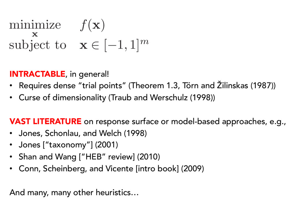
3. minimize x f (x) subject to x 2 [ 1 , 1] m INTRACTABLE, in general! •  Requires dense “trial points” (Theorem 1.3, Törn and Žilinskas (1987)) •  Curse of dimensionality (Traub and Werschulz (1998)) VAST LITERATURE on response surface or model-based approaches, e.g., •  Jones, Schonlau, and Welch (1998) •  Jones [“taxonomy”] (2001) •  Shan and Wang [“HEB” review] (2010) •  Conn, Scheinberg, and Vicente [intro book] (2009) And many, many other heuristics…
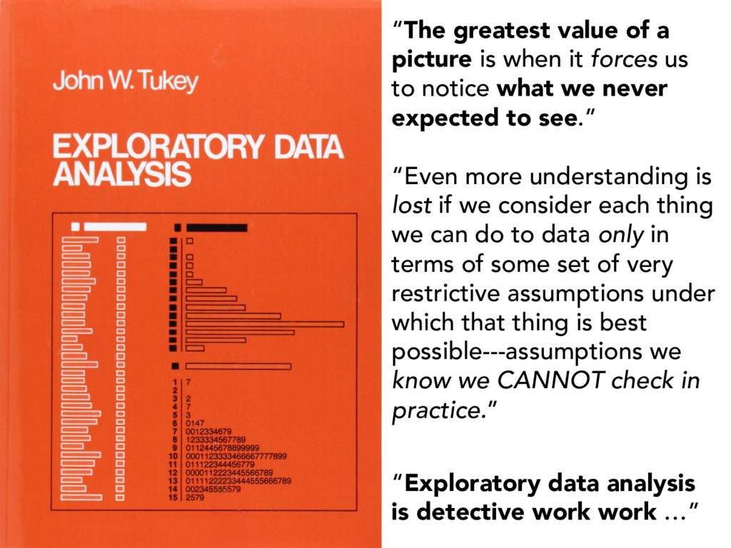
4. “The greatest value of a picture is when it forces us to notice what we never expected to see.” “Even more understanding is lost if we consider each thing we can do to data only in terms of some set of very restrictive assumptions under which that thing is best possible---assumptions we know we CANNOT check in practice.” “Exploratory data analysis is detective work work …”
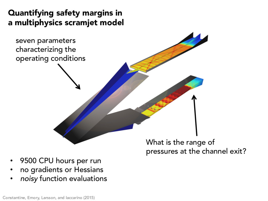
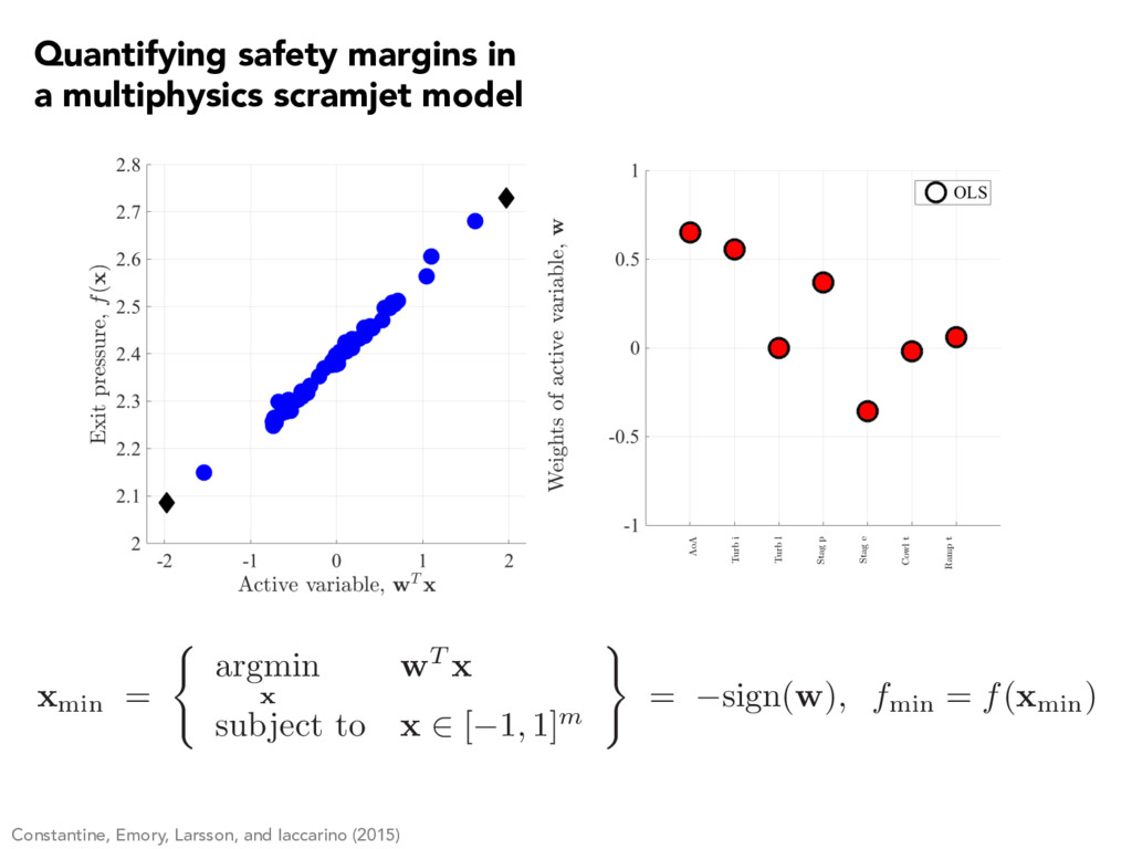
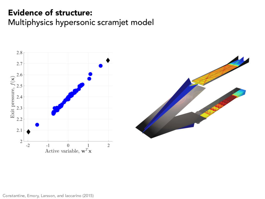
5. Constantine, Emory, Larsson, and Iaccarino (2015) •  9500 CPU hours per run •  no gradients or Hessians •  noisy function evaluations What is the range of pressures at the channel exit? seven parameters characterizing the operating conditions Quantifying safety margins in a multiphysics scramjet model
6. xmin = ( argmin x w T x subject to x 2 [ 1 , 1] m ) = sign(w) , fmin = f (xmin) Constantine, Emory, Larsson, and Iaccarino (2015) Quantifying safety margins in a multiphysics scramjet model
7. www.youtube.com/watch?v=mJvKzjT6lmY
8. youtu.be/Fek2HstkFVc Design a jet nozzle under uncertainty (DARPA SEQUOIA project) 10-parameter engine performance model Alonso, Eldred, Constantine et al. (2017)
9. IDEA Given , plot versus QUESTION How to get ? w f( x ) w T x w
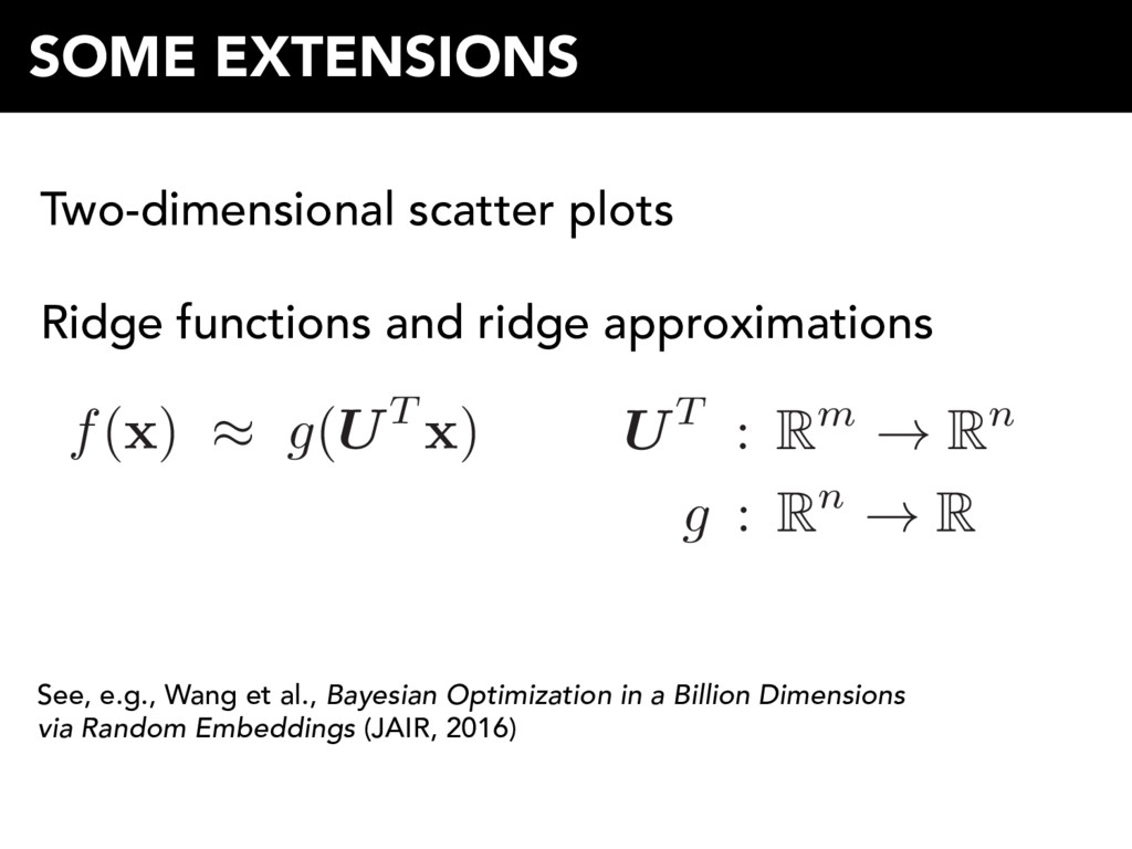
10. E [ ( I Cov[ x |f ]) 2 ] Cov[ E [ x |f ] ] f( x ) ⇡ a + b T x w = b / k b k How to get ? w Gradient of least-squares linear model [Li and Duan (1989)] Sliced Inverse Regression (SIR): first eigenvector of [Li (1991)] Sliced Average Variance Estimation (SAVE): first eigenvector of [Cook and Weisberg (1991)] Principal Hessian Directions (pHd): first eigenvector of [Li (1992)] E[ r2f( x ) ] Active Subspaces: first eigenvector of [Hristache et al. (2001), Constantine et al. (2014)] E[ rf( x ) rf( x )T ] Projection Pursuit Regression (PPR), Ridge Approximation [Friedman and Stuetzle (1981), Constantine et al. (2016)] min. w,g f( x ) g( w T x )
11. E [ ( I Cov[ x |f ]) 2 ] Cov[ E [ x |f ] ] f( x ) ⇡ a + b T x w = b / k b k How to get ? w Gradient of least-squares linear model [Li and Duan (1989)] Sliced Inverse Regression (SIR): first eigenvector of [Li (1991)] Sliced Average Variance Estimation (SAVE): first eigenvector of [Cook and Weisberg (1991)] Principal Hessian Directions (pHd): first eigenvector of [Li (1992)] E[ r2f( x ) ] Active Subspaces: first eigenvector of [Hristache et al. (2001), Constantine et al. (2014)] E[ rf( x ) rf( x )T ] Projection Pursuit Regression (PPR), Ridge Approximation [Friedman and Stuetzle (1981), Constantine et al. (2016)] min. w,g f( x ) g( w T x ) NOTES +  Maximizes squared correlation +  Cheap to fit -  Misses quadratic-like behavior
12. E [ ( I Cov[ x |f ]) 2 ] Cov[ E [ x |f ] ] f( x ) ⇡ a + b T x w = b / k b k How to get ? w Gradient of least-squares linear model [Li and Duan (1989)] Sliced Inverse Regression (SIR): first eigenvector of [Li (1991)] Sliced Average Variance Estimation (SAVE): first eigenvector of [Cook and Weisberg (1991)] Principal Hessian Directions (pHd): first eigenvector of [Li (1992)] E[ r2f( x ) ] Active Subspaces: first eigenvector of [Hristache et al. (2001), Constantine et al. (2014)] E[ rf( x ) rf( x )T ] Projection Pursuit Regression (PPR), Ridge Approximation [Friedman and Stuetzle (1981), Constantine et al. (2016)] min. w,g f( x ) g( w T x ) NOTES Methods for inverse regression
13. E [ ( I Cov[ x |f ]) 2 ] Cov[ E [ x |f ] ] f( x ) ⇡ a + b T x w = b / k b k How to get ? w Gradient of least-squares linear model [Li and Duan (1989)] Sliced Inverse Regression (SIR): first eigenvector of [Li (1991)] Sliced Average Variance Estimation (SAVE): first eigenvector of [Cook and Weisberg (1991)] Principal Hessian Directions (pHd): first eigenvector of [Li (1992)] E[ r2f( x ) ] Active Subspaces: first eigenvector of [Hristache et al. (2001), Constantine et al. (2014)] E[ rf( x ) rf( x )T ] Projection Pursuit Regression (PPR), Ridge Approximation [Friedman and Stuetzle (1981), Constantine et al. (2016)] min. w,g f( x ) g( w T x ) NOTES •  Known as sufficient dimension reduction •  See Cook, Regression Graphics (1998)
14. E [ ( I Cov[ x |f ]) 2 ] Cov[ E [ x |f ] ] f( x ) ⇡ a + b T x w = b / k b k How to get ? w Gradient of least-squares linear model [Li and Duan (1989)] Sliced Inverse Regression (SIR): first eigenvector of [Li (1991)] Sliced Average Variance Estimation (SAVE): first eigenvector of [Cook and Weisberg (1991)] Principal Hessian Directions (pHd): first eigenvector of [Li (1992)] E[ r2f( x ) ] Active Subspaces: first eigenvector of [Hristache et al. (2001), Constantine et al. (2014)] E[ rf( x ) rf( x )T ] Projection Pursuit Regression (PPR), Ridge Approximation [Friedman and Stuetzle (1981), Constantine et al. (2016)] min. w,g f( x ) g( w T x ) NOTES •  Two of four average derivative functionals from Samarov (1993) -  Require derivatives •  Use model-based derivative approximations, if derivatives not available
15. E [ ( I Cov[ x |f ]) 2 ] Cov[ E [ x |f ] ] f( x ) ⇡ a + b T x w = b / k b k How to get ? w Gradient of least-squares linear model [Li and Duan (1989)] Sliced Inverse Regression (SIR): first eigenvector of [Li (1991)] Sliced Average Variance Estimation (SAVE): first eigenvector of [Cook and Weisberg (1991)] Principal Hessian Directions (pHd): first eigenvector of [Li (1992)] E[ r2f( x ) ] Active Subspaces: first eigenvector of [Hristache et al. (2001), Constantine et al. (2014)] E[ rf( x ) rf( x )T ] Projection Pursuit Regression (PPR), Ridge Approximation [Friedman and Stuetzle (1981), Constantine et al. (2016)] min. w,g f( x ) g( w T x ) NOTES Not all eigenvector- based techniques are PCA!
16. E [ ( I Cov[ x |f ]) 2 ] Cov[ E [ x |f ] ] f( x ) ⇡ a + b T x w = b / k b k How to get ? w Gradient of least-squares linear model [Li and Duan (1989)] Sliced Inverse Regression (SIR): first eigenvector of [Li (1991)] Sliced Average Variance Estimation (SAVE): first eigenvector of [Cook and Weisberg (1991)] Principal Hessian Directions (pHd): first eigenvector of [Li (1992)] E[ r2f( x ) ] Active Subspaces: first eigenvector of [Hristache et al. (2001), Constantine et al. (2014)] E[ rf( x ) rf( x )T ] Projection Pursuit Regression (PPR), Ridge Approximation [Friedman and Stuetzle (1981), Constantine et al. (2016)] min. w,g f( x ) g( w T x ) NOTES •  Related to neural nets; see Hastie et al. ESL (2009) •  Different from ridge recovery; see Fornasier et al. (2012)
17. E [ ( I Cov[ x |f ]) 2 ] Cov[ E [ x |f ] ] f( x ) ⇡ a + b T x w = b / k b k How to get ? w Gradient of least-squares linear model [Li and Duan (1989)] Sliced Inverse Regression (SIR): first eigenvector of [Li (1991)] Sliced Average Variance Estimation (SAVE): first eigenvector of [Cook and Weisberg (1991)] Principal Hessian Directions (pHd): first eigenvector of [Li (1992)] E[ r2f( x ) ] Active Subspaces: first eigenvector of [Hristache et al. (2001), Constantine et al. (2014)] E[ rf( x ) rf( x )T ] Projection Pursuit Regression (PPR), Ridge Approximation [Friedman and Stuetzle (1981), Constantine et al. (2016)] min. w,g f( x ) g( w T x ) Regression or approximation? NOTES Glaws, Constantine, and Cook (2017)
18. So you found … QUESTION Is it any good? w
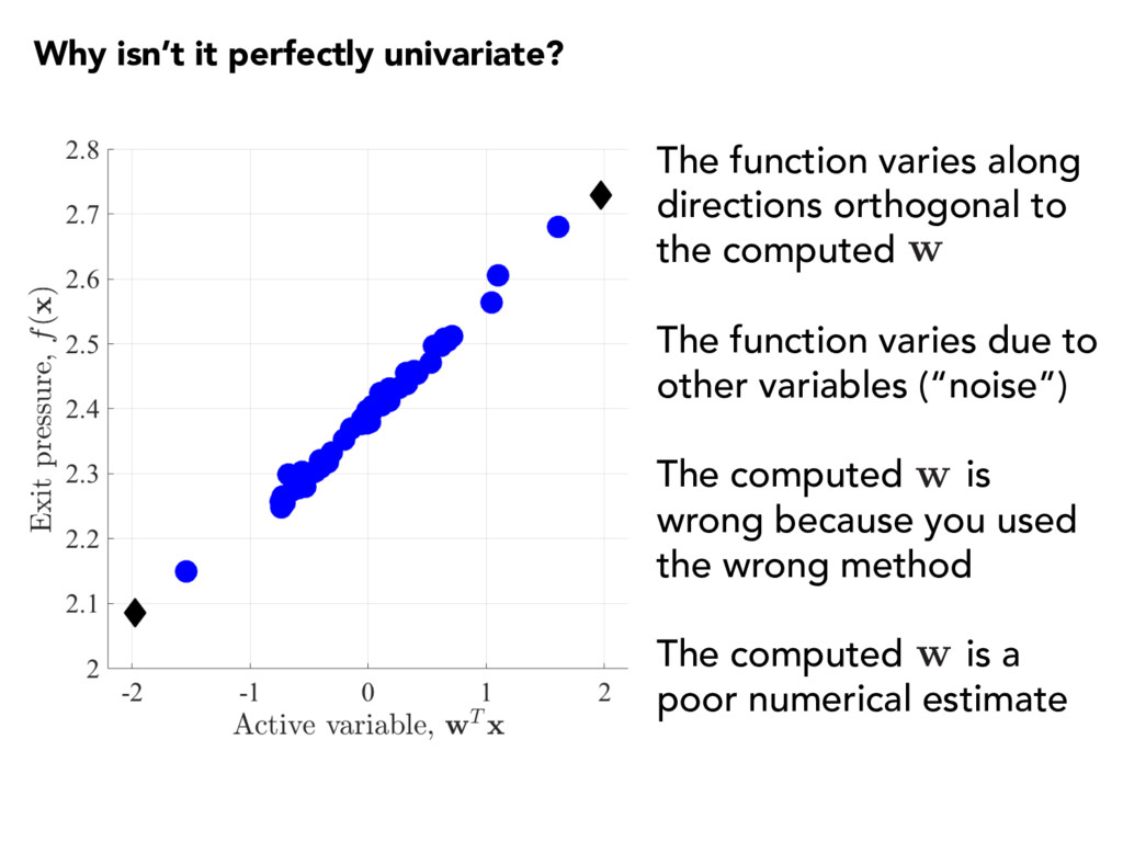
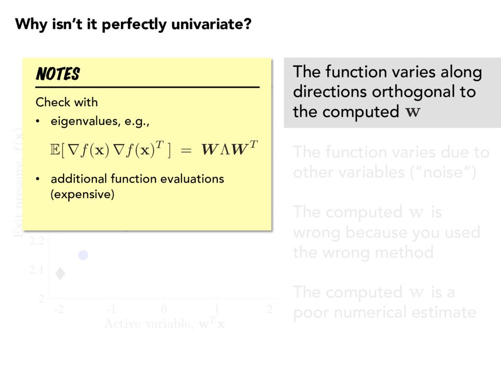
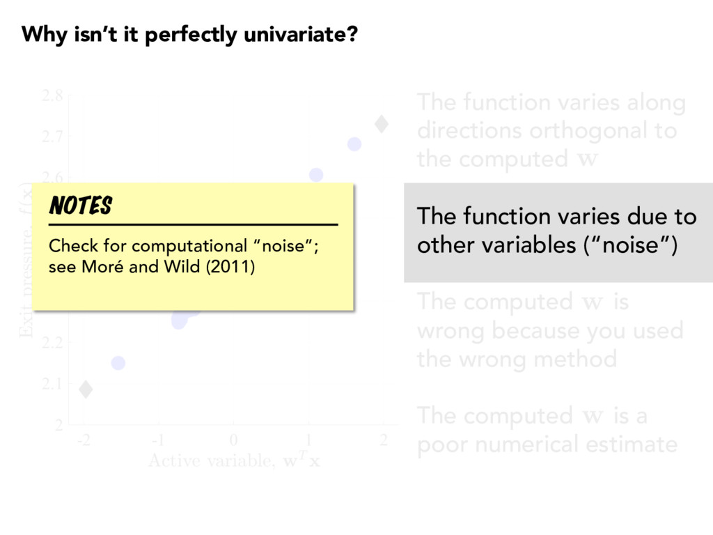
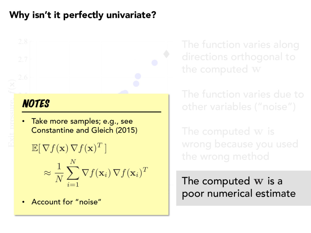
19. Why isn’t it perfectly univariate? The function varies along directions orthogonal to the computed The function varies due to other variables (“noise”) The computed is wrong because you used the wrong method The computed is a poor numerical estimate w w w
20. Why isn’t it perfectly univariate? The function varies along directions orthogonal to the computed The function varies due to other variables (“noise”) The computed is wrong because you used the wrong method The computed is a poor numerical estimate w w w NOTES Check with •  eigenvalues, e.g., •  additional function evaluations (expensive) E[ rf( x ) rf( x )T ] = W ⇤W T
21. Why isn’t it perfectly univariate? The function varies along directions orthogonal to the computed The function varies due to other variables (“noise”) The computed is wrong because you used the wrong method The computed is a poor numerical estimate w w w NOTES Check for computational “noise”; see Moré and Wild (2011)
22. Why isn’t it perfectly univariate? The function varies along directions orthogonal to the computed The function varies due to other variables (“noise”) The computed is wrong because you used the wrong method The computed is a poor numerical estimate w w w NOTES Try multiple approaches for computing , if possible w
23. Why isn’t it perfectly univariate? The function varies along directions orthogonal to the computed The function varies due to other variables (“noise”) The computed is wrong because you used the wrong method The computed is a poor numerical estimate w w w NOTES •  Take more samples; e.g., see Constantine and Gleich (2015) •  Account for “noise” E[ rf( x ) rf( x )T ] ⇡ 1 N N X i=1 rf( xi) rf( xi)T
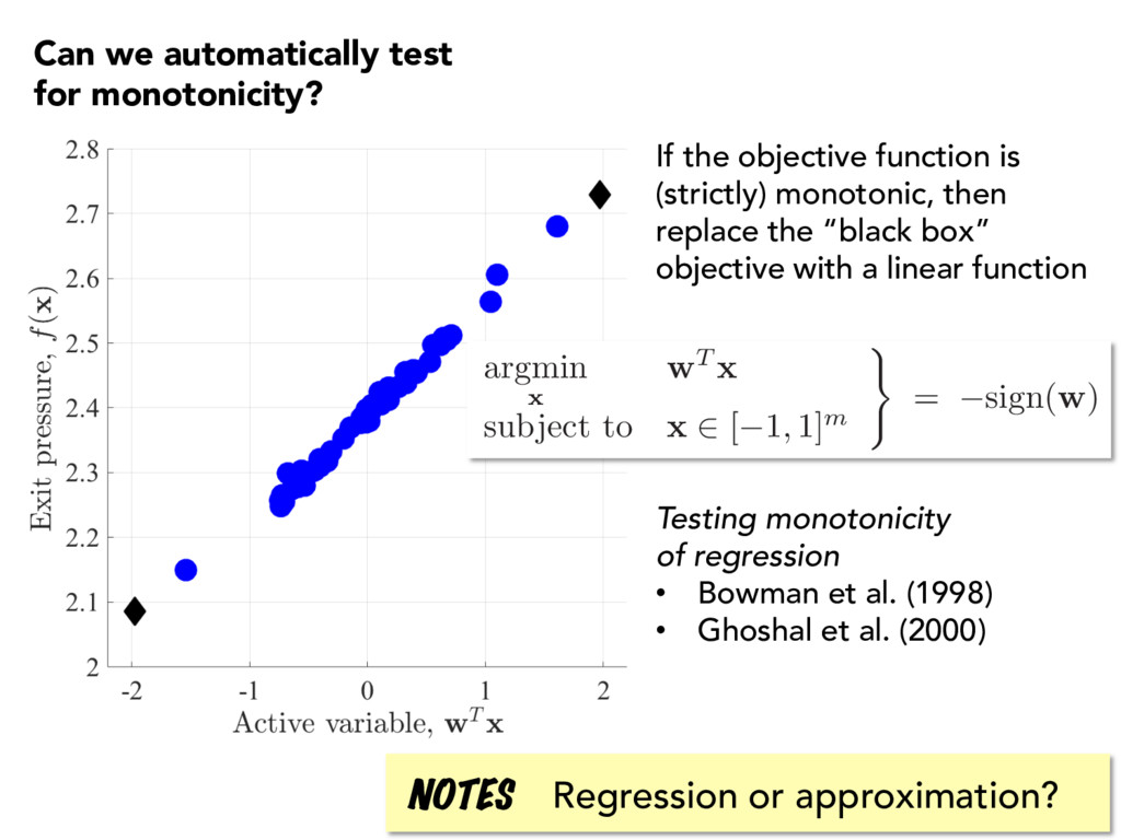
24. If the objective function is (strictly) monotonic, then replace the “black box” objective with a linear function Testing monotonicity of regression •  Bowman et al. (1998) •  Ghoshal et al. (2000) Regression or approximation? NOTES Can we automatically test for monotonicity? argmin x w T x subject to x 2 [ 1 , 1] m ) = sign(w)
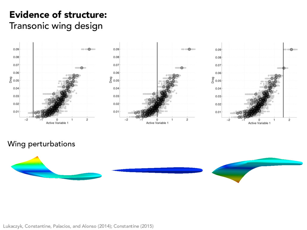
25. Sensitivity of linear program solution Constantine, Emory, Larsson, and Iaccarino (2015) -1 0 1 0 0.05 0.1 AoA -1 0 1 0 0.05 0.1 Turb int -1 0 1 0 0.05 0.1 Turb len -1 0 1 0 0.05 0.1 Stag pres -1 0 1 0 0.05 0.1 Stag enth -1 0 1 0 0.05 0.1 Cowl trans -1 0 1 0 0.05 0.1 Ramp trans Use a bootstrap (sampling with replacement) to assess sensitivity of weights with respect to the “data” NOTES Weight close to zero indicates •  high sensitivity in minimizer •  low sensitivity in minimum Weight can give sensitivity information; see Constantine and Diaz (2017)
26. Do real world models have such structure?
27. Constantine, Emory, Larsson, and Iaccarino (2015) Evidence of structure: Multiphysics hypersonic scramjet model
28. Jefferson, Gilbert, Constantine, and Maxwell (2015); Jefferson, Constantine, and Maxwell (2017) Evidence of structure: Integrated hydrologic model
29. Lukaczyk, Constantine, Palacios, and Alonso (2014); Constantine (2015) Evidence of structure: Transonic wing design Wing perturbations
30. T-cell count Loudon and Pankavich (2017) Evidence of structure: In-host HIV dynamics
31. −2 −1 0 1 2 0 0.05 0.1 0.15 0.2 0.25 Active Variable 1 P max (watts) Constantine, Zaharatos, and Campanelli (2015) Evidence of structure: Solar-cell circuit model
32. −1.5 −1.0 −0.5 0.0 0.5 1.0 1.5 Active variable 4000 5000 6000 7000 8000 9000 10000 Stagnation pressure Cortesi, Constantine, Magin, and Congedo (In prep.) Evidence of structure: Atmospheric re-entry vehicle
33. -1 0 1 wT 1 x 0 5 10 15 f(x) Average velocity Glaws, Constantine, Shadid, and Wildey (2017) Evidence of structure: Magnetohydrodynamics generator model
34. 2 0 2 wT x 3.2 3.4 3.6 Voltage [V] Constantine and Doostan (2017) Evidence of structure: Lithium-ion battery model
35. Othmer, Lukaczyk, Constantine, and Alonso (2016) Evidence of structure: Automobile design
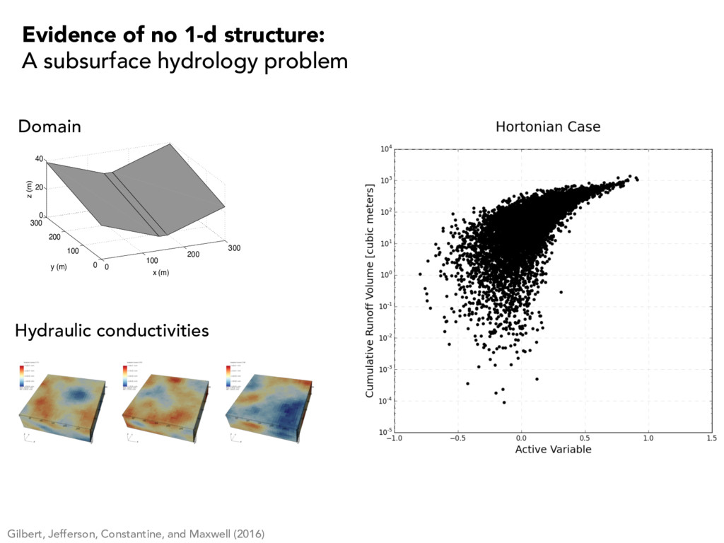
36. Gilbert, Jefferson, Constantine, and Maxwell (2016) Evidence of no 1-d structure: A subsurface hydrology problem 0 100 200 300 0 100 200 300 0 20 40 x (m) y (m) z (m) Student Version of MATLAB Domain Hydraulic conductivities
37. Jupyter notebooks: github.com/paulcon/as-data-sets
38. WHY IS THIS HAPPENING??? Here’s my hunch … (1) monotonicity (2) small range of parameters
39. SOME EXTENSIONS Two-dimensional scatter plots Ridge functions and ridge approximations f( x ) ⇡ g(UT x ) UT : Rm ! Rn g : Rn ! R See, e.g., Wang et al., Bayesian Optimization in a Billion Dimensions via Random Embeddings (JAIR, 2016)
40. www.siam.org/meetings/dr17/
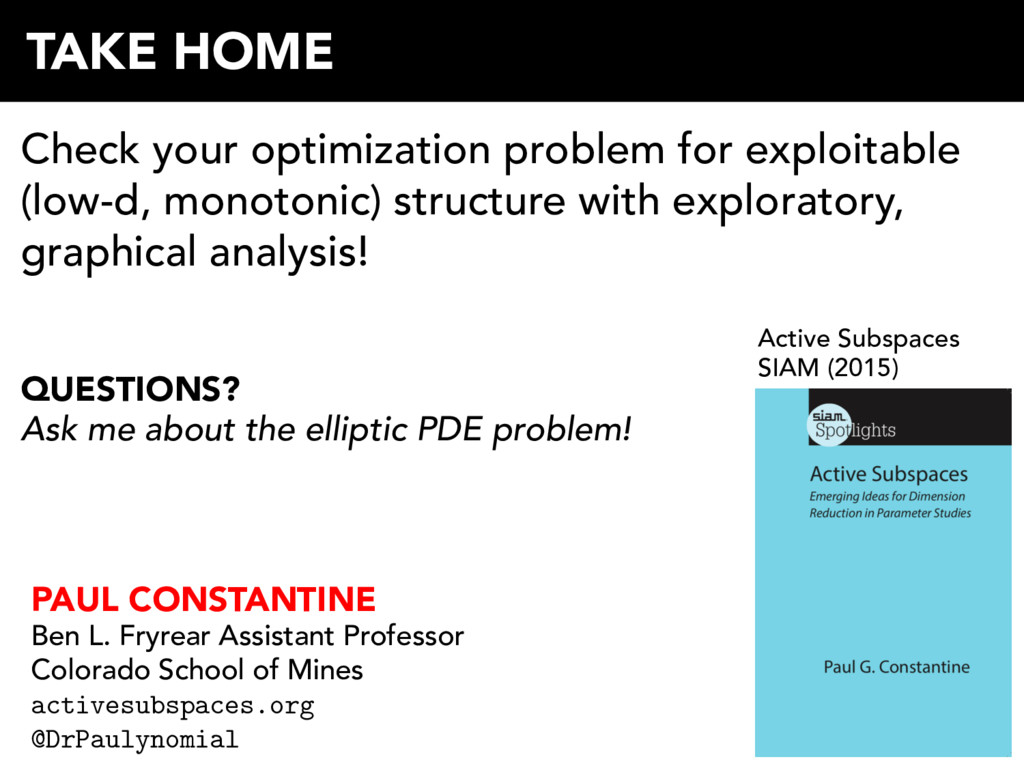
41. PAUL CONSTANTINE Ben L. Fryrear Assistant Professor Colorado School of Mines activesubspaces.org! @DrPaulynomial! TAKE HOME Active Subspaces SIAM (2015) Check your optimization problem for exploitable (low-d, monotonic) structure with exploratory, graphical analysis! QUESTIONS? Ask me about the elliptic PDE problem!
42. BACK UP SLIDES
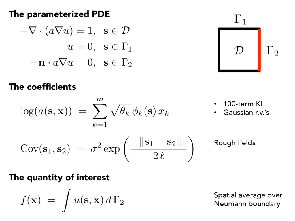
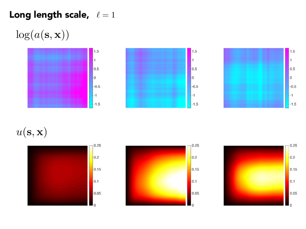
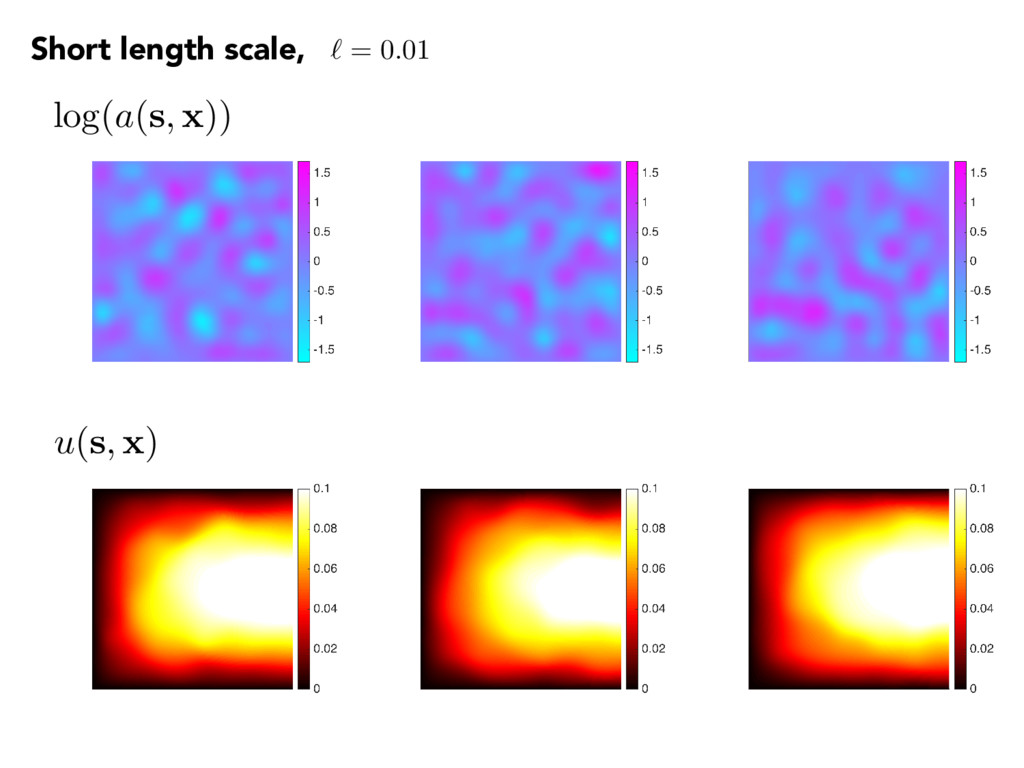
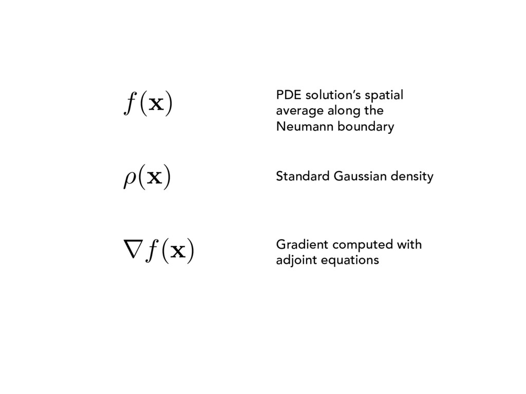
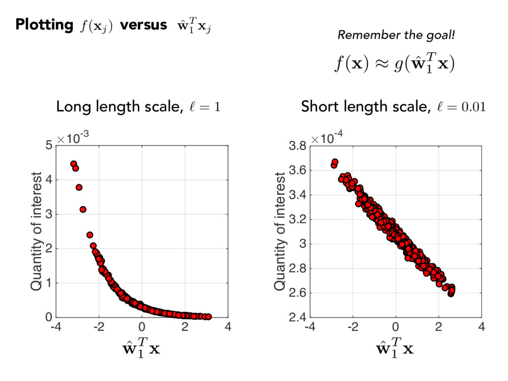
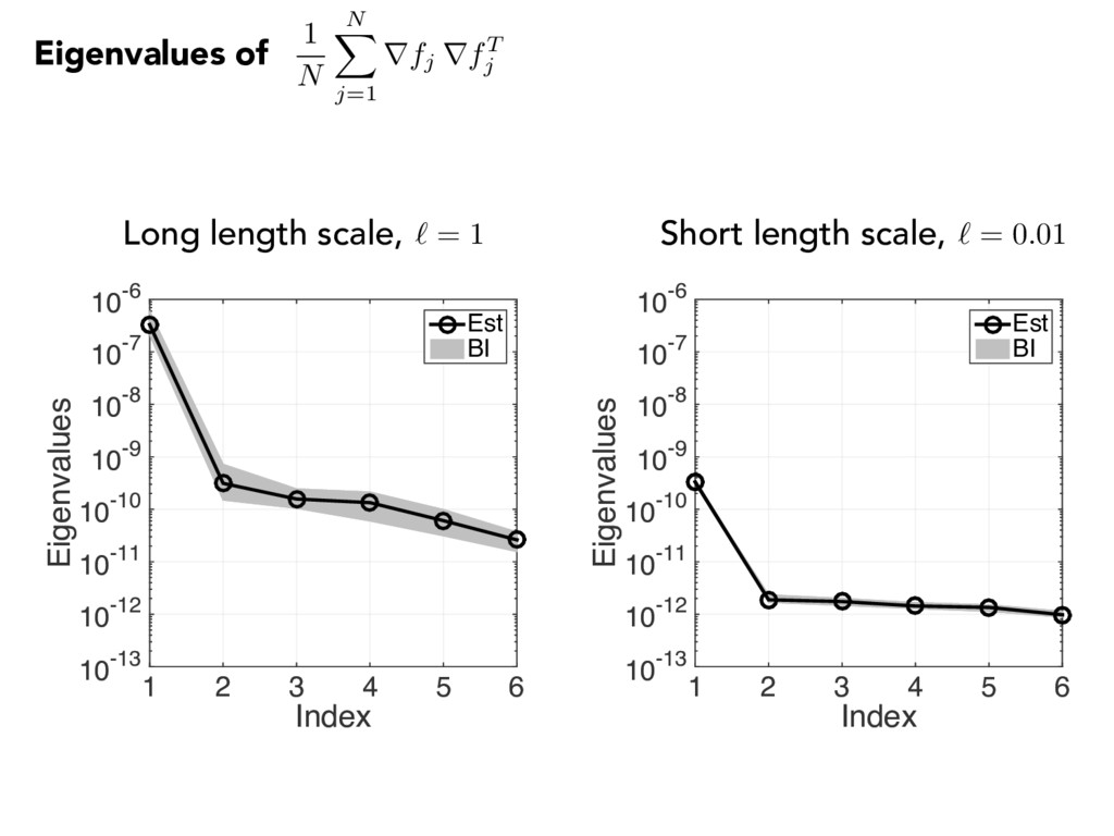
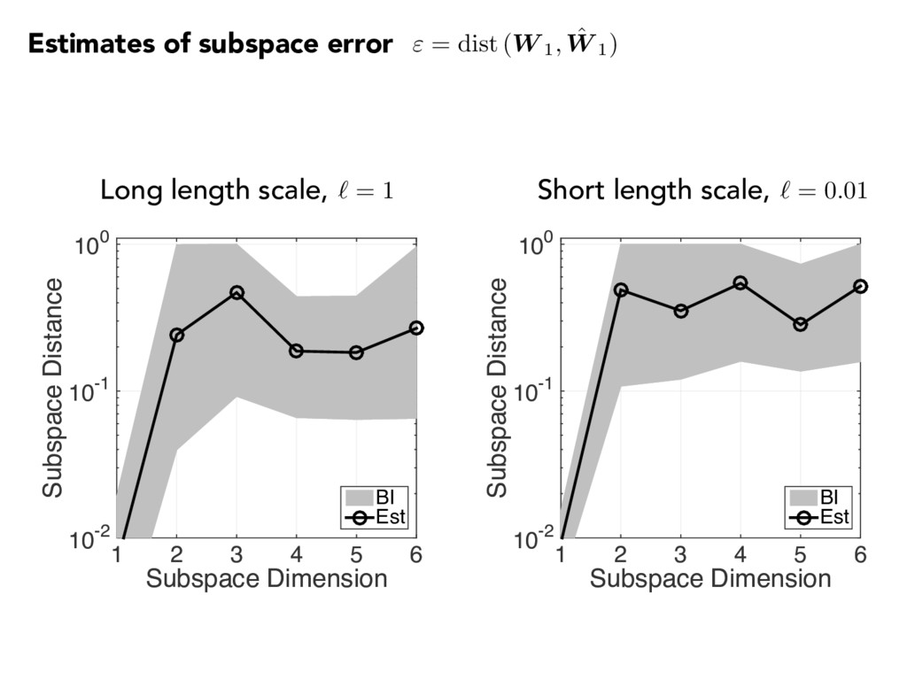
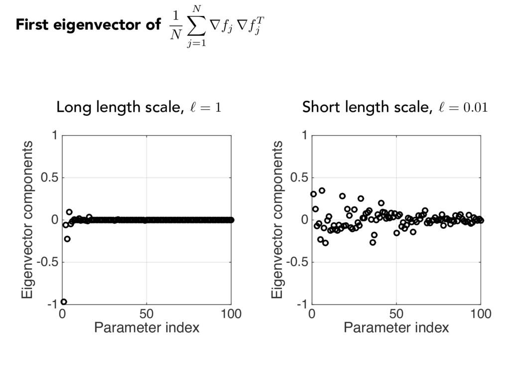
43. D 1 2 The parameterized PDE The coefficients r · (aru) = 1, s 2 D u = 0, s 2 1 n · aru = 0, s 2 2 log(a(s, x)) = m X k=1 p ✓k k(s) xk Cov( s1, s2) = 2 exp ✓ ks1 s2 k1 2 ` ◆ The quantity of interest f( x ) = Z u( s , x ) d 2 •  100-term KL •  Gaussian r.v.’s Rough fields Spatial average over Neumann boundary
44. Long length scale, ` = 1 log( a (s , x)) u( s , x )
45. Short length scale, log( a (s , x)) u( s , x ) ` = 0.01
46. f( x ) ⇢( x ) rf( x ) PDE solution’s spatial average along the Neumann boundary Standard Gaussian density Gradient computed with adjoint equations
47. -4 -2 0 2 4 Quantity of interest #10-3 0 1 2 3 4 5 -4 -2 0 2 4 Quantity of interest #10-4 2.4 2.6 2.8 3 3.2 3.4 3.6 3.8 Long length scale, ` = 1 Short length scale, ` = 0.01 f( x ) ⇡ g( ˆ w T 1 x ) ˆ w T 1 x ˆ w T 1 x Remember the goal! Plotting versus f( xj) ˆ w T 1 xj
48. Index 1 2 3 4 5 6 Eigenvalues 10-13 10-12 10-11 10-10 10-9 10-8 10-7 10-6 Est BI Index 1 2 3 4 5 6 Eigenvalues 10-13 10-12 10-11 10-10 10-9 10-8 10-7 10-6 Index 1 2 3 4 5 6 Eigenvalues 10-13 10-12 10-11 10-10 10-9 10-8 10-7 10-6 Est BI Index 1 2 3 4 5 6 Eigenvalues 10-13 10-12 10-11 10-10 10-9 10-8 10-7 10-6 Long length scale, ` = 1 Short length scale, ` = 0.01 Eigenvalues of 1 N N X j=1 rfj rfT j
49. Subspace Dimension 1 2 3 4 5 6 Subspace Distance 10-2 10-1 100 BI Est Subspace Dimension 1 2 3 4 5 6 Subspace Distance 10-2 10-1 100 Subspace Dimension 1 2 3 4 5 6 Subspace Distance 10-2 10-1 100 BI Est Subspace Dimension 1 2 3 4 5 6 Subspace Distance 10-2 10-1 100 Long length scale, ` = 1 Short length scale, ` = 0.01 Estimates of subspace error " = dist (W 1, ˆ W 1)
50. Parameter index 0 50 100 Eigenvector components -1 -0.5 0 0.5 1 Parameter index 0 50 100 Eigenvector components -1 -0.5 0 0.5 1 First eigenvector of Long length scale, ` = 1 Short length scale, ` = 0.01 1 N N X j=1 rfj rfT j